
Spur gears are among the most widely used machine elements for power transmission in modern industrial equipment. Their meshing stability and fatigue resistance directly determine the reliability, transmission efficiency, and smoothness of the whole system. Single-stage spur gears are often preferred because of their simple geometry and high efficiency. They are used in high-speed train gearboxes, reducer sets, couplings, wind turbines, and many other rotating machines. In my research, I focus on the interaction between the elastohydrodynamic lubrication (EHL) characteristics and the nonlinear dynamic response of single-stage spur gears. I combine theoretical modeling, numerical simulation, continuation shooting techniques, and cell-mapping methods to investigate the stability of coexisting attractors, the transition processes induced by bifurcations, and the influence of lubrication conditions on chaotic behavior.
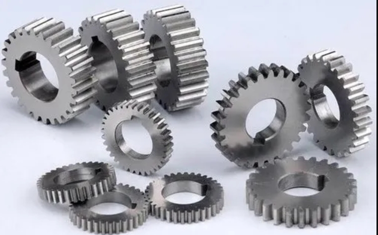
The central problem addressed in this study is that high-speed and heavy-load conditions cause the lubricant film between meshing teeth of spur gears to become very thin. If the film ruptures, tooth surface pitting, scuffing, and severe vibration may occur. Traditional gear dynamics models often neglect the oil-film stiffness or treat the mesh stiffness as a purely structural quantity. In real single-stage spur gears, however, the oil film and the tooth deformation act like two springs in series. Therefore, the comprehensive time-varying mesh stiffness differs from the dry contact stiffness. This difference changes the bifurcation structure and the coexisting attractors of the gear system. In the following sections, I present a complete study from lubrication theory to nonlinear dynamics, with special attention to the stability boundaries of spur gears under normal and starved lubrication.
1. Introduction and Scope of the Research
The rapid development of rail transportation has significantly increased the operating speed of gear transmission systems. Modern electric multiple units require gearboxes to operate reliably at high rotational speeds and over a wide temperature range. Under such extreme conditions, the lubricant film between the tooth surfaces of spur gears is subjected to high pressure, high shear rate, and transient loading. The classical Reynolds equation cannot directly describe the elastic deformation of the tooth surfaces, and therefore an elastohydrodynamic lubrication model is needed. EHL theory couples the hydrodynamic pressure generation with the elastic deformation of the contact solids. For spur gears, the contact along the tooth width can be approximated as a line contact. This approximation is widely accepted because the face width is usually much larger than the contact half-width.
The main goals of my research are as follows. First, I establish a line-contact EHL model and solve the pressure and film-thickness distributions for meshing spur gears. Second, I compute the geometric and kinematic parameters along the line of action, including the curvature radii, sliding velocity, rolling velocity, and normal load. Third, I analyze how operating conditions, such as speed, torque, lubricant viscosity, and pressure-viscosity coefficient, affect the EHL characteristics of spur gears. Fourth, I build a combined stiffness model that includes both the tooth contact stiffness and the oil-film stiffness. Finally, I insert the time-varying comprehensive stiffness into a single-degree-of-freedom nonlinear dynamic model of single-stage spur gears. Using continuation shooting and basin-of-attraction methods, I study the coexisting attractors, their stability, and their bifurcation transitions under both adequate lubrication and starved lubrication.
2. Line-Contact Elastohydrodynamic Lubrication Theory
The line-contact EHL model converts a meshing spur gear pair into an equivalent elastic cylinder pressed against a rigid plane. The equivalent cylinder has the combined curvature radius of the two gears. The normal load deforms the elastic body, and the lubricant is entrained into the contact by the surface velocities. This model is governed by five fundamental equations: the Reynolds equation, the film-thickness equation, the viscosity-pressure equation, the density-pressure equation, and the load balance equation.
The steady-state one-dimensional Reynolds equation for line-contact EHL is
$$ \frac{\partial}{\partial x}\left(\frac{\rho h^3}{12\eta}\frac{\partial p}{\partial x}\right)
= \frac{u_s}{2}\frac{\partial(\rho h)}{\partial x}, $$
where \(p\) is the lubricant pressure, \(h\) is the local film thickness, \(\eta\) is the dynamic viscosity, \(\rho\) is the lubricant density, and \(u_s\) is the entrainment or rolling velocity. In the dimensionless form, the Reynolds equation becomes
$$ \frac{\partial}{\partial X}\left(\varepsilon \frac{\partial P}{\partial X}\right)
= \frac{\partial(\bar{\rho} H)}{\partial X}, $$
with
$$ \varepsilon=\frac{\bar{\rho} H^3}{\bar{\eta}\lambda},
\qquad
\lambda=\frac{12\eta_0 u_s E’ R^2}{b^3 p_H}, $$
where \(X\), \(P\), \(H\), \(\bar{\rho}\), and \(\bar{\eta}\) are the dimensionless coordinate, pressure, film thickness, density, and viscosity, respectively.
The dimensionless film-thickness equation is
$$ H(X)=H_0+\frac{X^2}{2}
-\frac{1}{\pi}\int_{X_{\rm in}}^{X_{\rm out}} P(X’)\ln|X-X’|\,dX’, $$
where \(H_0\) is the rigid-body separation and the integral term represents the elastic deformation of the tooth surfaces. The viscosity-pressure relation is based on the Roelands equation:
$$ \bar{\eta}
=\exp\left\{(\ln\eta_0+9.67)\left[\left(1+5.1\times10^{-9}p\right)^z-1\right]\right\}, $$
and the compressibility of the lubricant is described by
$$ \bar{\rho}=1+\frac{0.6\times10^{-9}p}{1+1.7\times10^{-9}p}. $$
The pressure distribution must satisfy the load balance equation, which in dimensionless form is written as
$$ \int_{X_{\rm in}}^{X_{\rm out}}P\,dX=\frac{\pi}{2}. $$
I solve these equations by a finite-difference method. The computational domain is divided into equally spaced nodes, typically 130 nodes from \(X_{\rm in}=-4\) to \(X_{\rm out}=1.2\). The pressure convergence criterion is chosen as \(10^{-6}\). The computed pressure and film-thickness distributions show two well-known EHL features: the second pressure peak and the film-thickness necking near the outlet. The second pressure peak appears because the sudden expansion of the outlet gap reduces the elastic deformation, causing the film to contract. The lubricant is then forced through a converging channel, which generates a local pressure rise. At the same location, the film thickness reaches its minimum value. This behavior is essential for understanding the lubrication state of spur gears because the minimum film thickness determines whether the tooth surfaces are separated by a continuous oil film or enter the mixed or boundary lubrication regime.
The following table summarizes the lubricant and contact parameters used in the line-contact EHL simulation.
| Parameter | Symbol | Value |
|---|---|---|
| Contact load per unit width | \(w\) | \(1\times10^5\ \mathrm{N/m}\) |
| Entrainment velocity | \(u_s\) | \(1\ \mathrm{m/s}\) |
| Equivalent radius | \(R\) | \(0.015\ \mathrm{m}\) |
| Equivalent elastic modulus | \(E’\) | \(2.2\times10^{11}\ \mathrm{Pa}\) |
| Ambient viscosity | \(\eta_0\) | \(0.06\ \mathrm{Pa\cdot s}\) |
| Pressure-viscosity coefficient | \(\alpha\) | \(22.6\ \mathrm{GPa^{-1}}\) |
| Lubricant density | \(\rho_0\) | \(910\ \mathrm{kg/m^3}\) |
3. Geometric and Kinematic Analysis of Spur Gears
To study the lubrication characteristics of single-stage spur gears, I first establish the geometric model of the meshing pair. The two gears are assumed to be standard involute spur gears. The main parameters are listed below.
| Parameter | Symbol | Value |
|---|---|---|
| Number of teeth | \(z_1,z_2\) | 36, 40 |
| Module | \(m\) | 2 mm |
| Pressure angle | \(\alpha\) | 20° |
| Addendum coefficient | \(h_a^*\) | 1.0 |
| Face width | \(B\) | 40 mm |
| Pinion torque | \(T_1\) | 600 N·m |
| Pinion speed | \(n_1\) | 2000 rpm |
| Equivalent elastic modulus | \(E’\) | 2.2×10¹¹ Pa |
| Lubricant ambient viscosity | \(\eta_0\) | 0.075 Pa·s |
| Pressure-viscosity coefficient | \(\alpha\) | 1.96×10⁻⁸ Pa-1 |
The involute meshing condition with no backlash is expressed as
$$ \operatorname{inv}\alpha’
= \frac{2(x_1+x_2)}{z_1+z_2}\tan\alpha+\operatorname{inv}\alpha, $$
where \(\operatorname{inv}\alpha=\tan\alpha-\alpha\), \(x_1\) and \(x_2\) are profile shift coefficients, and \(\alpha’\) is the operating pressure angle. The pitch radii and base radii of the two gear wheels are
$$ R_{p1}=\frac{mz_1}{2}\frac{\cos\alpha}{\cos\alpha’},\qquad
R_{p2}=\frac{mz_2}{2}\frac{\cos\alpha}{\cos\alpha’}, $$
$$ R_{b1}=\frac{mz_1}{2}\cos\alpha,\qquad
R_{b2}=\frac{mz_2}{2}\cos\alpha. $$
During meshing, the instantaneous contact point moves along the line of action. If \(\xi\) is the distance from the pitch point to the current contact point, the local curvature radii of the pinion and gear are
$$ R_1=R_{p1}\sin\alpha’-\xi,\qquad
R_2=R_{p2}\sin\alpha’+\xi. $$
The combined curvature radius is
$$ R=\frac{R_1R_2}{R_1+R_2}. $$
The surface velocities of the pinion and gear at the contact point are
$$ u_1=\frac{\pi n_1}{30}R_1,\qquad
u_2=\frac{\pi n_2}{30}R_2. $$
The rolling velocity \(u_r\) and the sliding velocity \(u_s\) are defined as
$$ u_r=\frac{u_1+u_2}{2},\qquad
u_s=|u_1-u_2|. $$
At the pitch point, the sliding velocity is zero. Before the pitch point, the gear velocity is larger than the pinion velocity; after the pitch point, the pinion velocity exceeds the gear velocity. This velocity reversal directly influences the entrainment and shear of the oil film. The normal load per unit length along the line of action changes abruptly when the meshing state switches from double-tooth contact to single-tooth contact. During double-tooth contact, the load is shared by two pairs of teeth, so the unit load is lower. During single-tooth contact, the load per unit width jumps to a higher value. These load variations produce significant changes in the EHL pressure and film thickness of spur gears.
3.1 Influence of Rotational Speed on the Lubrication of Spur Gears
I first investigate the effect of pinion speed. Three speeds are considered: 1500 rpm, 2000 rpm, and 2500 rpm. With increasing speed, the entrainment velocity increases. The hydrodynamic pressure generated inside the oil film becomes larger, and the second pressure peak moves toward the inlet direction. The minimum film thickness also increases with speed. This means that high-speed operation of spur gears tends to produce a thicker oil film, which is beneficial for preventing direct metallic contact. However, the high sliding velocity also increases the oil temperature and the shear rate, so the effective viscosity may decrease in a full thermal EHL analysis.
3.2 Influence of Torque on the Lubrication of Spur Gears
I then examine the effect of external torque. The torque values are 100 N·m, 200 N·m, and 500 N·m. As the torque increases, the contact load increases, and the oil film pressure rises. The second pressure peak increases, and the minimum film thickness decreases. A thinner film makes the lubrication state more fragile. At low torque, the oil film is thicker and more stable. Therefore, torque is one of the most important operating parameters for the lubrication reliability of spur gears.
3.3 Influence of Viscosity and Pressure-Viscosity Coefficient
The ambient viscosity of the lubricant has a strong influence. I test \(\eta_0=0.04\), \(0.08\), and \(0.12\ \mathrm{Pa\cdot s}\). With higher viscosity, the oil film can sustain higher pressure, the second pressure peak becomes more pronounced, and the film thickness increases. The position of the second pressure peak moves away from the outlet. The necking area becomes thicker as well. The pressure-viscosity coefficient is also important. For \(\alpha=19.6\), \(22.6\), and \(32.6\ \mathrm{GPa^{-1}}\), the second pressure peak and the minimum film thickness increase markedly at the largest coefficient. This indicates that lubricants with a high pressure-viscosity coefficient can maintain effective lubrication of spur gears under high contact pressure.
4. Stiffness Modeling of Lubricated Spur Gears
The nonlinear dynamic behavior of spur gears is strongly affected by the time-varying mesh stiffness. I use the Ishikawa formula to calculate the tooth deformation. The tooth is idealized as a combination of a rectangular cantilever and a trapezoidal cantilever. The total deformation consists of five components:
$$ \delta=\delta_{br}+\delta_{bt}+\delta_s+\delta_p+\delta_g, $$
where \(\delta_{br}\) is the bending deformation of the rectangular part, \(\delta_{bt}\) is the bending deformation of the trapezoidal part, \(\delta_s\) is the shear deformation, \(\delta_p\) is the local contact deformation, and \(\delta_g\) is the deformation of the gear body. The meshing stiffness is then obtained from
$$ k_j(t)=\frac{F_n}{\delta}, $$
where \(F_n\) is the normal tooth load. The result is a periodic function because the meshing alternates between single-tooth contact and double-tooth contact. In the single-tooth contact zone, the stiffness is lower because the entire load is carried by one pair of teeth. In the double-tooth contact zone, the load is shared, the deformation is reduced, and the stiffness is higher.
The oil-film stiffness is calculated with two approaches. The first approach is based on the Dowson-Higginson empirical formulas for the central and minimum film thickness:
$$ h_c=3.06 U^{0.69} G^{0.56} W^{-0.10} R, $$
$$ h_m=2.65 U^{0.70} G^{0.54} W^{-0.13} R, $$
where \(U\), \(G\), and \(W\) are the dimensionless speed, material, and load parameters. From these formulas, the oil-film stiffness can be expressed as
$$ k_c=\frac{F}{0.1h_c}=\frac{10F}{h_c}, $$
$$ k_m=\frac{F}{0.13h_m}\approx \frac{7.69F}{h_m}. $$
The second approach is a global numerical method. The contact region is divided into small nodes, and the local oil-film stiffness at each node is
$$ k_{oj}=L\Delta x\frac{p_j}{h_j}\frac{R}{b}, $$
where \(p_j\) and \(h_j\) are the dimensionless pressure and film thickness at node \(j\), \(L\) is the face width, \(\Delta x\) is the grid length, \(R\) is the combined curvature radius, and \(b\) is the Hertzian contact half-width. The total oil-film stiffness is the sum of all local stiffness values.
The comprehensive time-varying stiffness of lubricated spur gears is obtained by connecting the tooth contact stiffness and the oil-film stiffness in series:
$$ k_z(t)=\left(\frac{1}{k_j(t)}+\frac{1}{k_o(t)}\right)^{-1}. $$
Because the oil-film stiffness is usually larger than the tooth contact stiffness, the comprehensive stiffness is slightly smaller than the dry contact stiffness. In the single-tooth contact zone, the oil-film stiffness is large; in the double-tooth contact zone, the comprehensive stiffness changes abruptly. To use the stiffness function in the nonlinear dynamic model, I fit the numerical data with a first-order Fourier series:
$$ k_z(t)=k_{av}+k_{ha}\cos(\omega t+\varphi), $$
where \(k_{av}\) is the average stiffness, \(k_{ha}\) is the harmonic amplitude, \(\omega\) is the meshing frequency, and \(\varphi\) is the phase angle.
For the starved lubrication condition, I assume that the minimum film thickness falls below 0.1 μm. In that regime, the film thickness ratio is below unity, which corresponds to boundary lubrication. The oil film cannot separate the rough surfaces completely. The contact pressure is partly supported by the asperities. I compute the oil-film stiffness under this reduced film thickness and obtain the starved comprehensive stiffness curve. Compared with the fully lubricated case, the starved stiffness is closer to the dry contact stiffness and fluctuates more severely. This creates stronger parametric excitation and may lead to more chaotic behavior in spur gears.
5. Nonlinear Dynamic Model and Continuation Shooting Method
The dynamic model of a single-degree-of-freedom spur gear pair is shown conceptually as a pair of rotating disks connected by a spring-damper element. The spring represents the time-varying mesh stiffness, including the oil-film stiffness, and the damper represents the mesh damping. The backlash function \(f(x)\) describes the loss of contact when the relative displacement is smaller than the backlash gap. The torsional equations of motion are reduced to one relative displacement coordinate:
$$ x=r_1\theta_1-r_2\theta_2-e(t), $$
where \(r_1\) and \(r_2\) are the base radii, \(\theta_1\) and \(\theta_2\) are the angular displacements, and \(e(t)\) is the static transmission error. The dimensionless equation of motion is
$$ \ddot{X}+2\zeta\dot{X}+K(\tau)f(X)
= F_m+\varepsilon\omega^2\cos(\omega\tau), $$
where \(\zeta\) is the dimensionless damping ratio, \(K(\tau)\) is the dimensionless time-varying comprehensive stiffness, \(F_m\) is the mean excitation, \(\varepsilon\) is the static transmission error amplitude, and \(\omega\) is the dimensionless meshing frequency. The backlash function is
$$ f(X)=
\begin{cases}
X-D, & X>D,\\
0, & |X|\le D,\\
X+D, & X<-D.
\end{cases} $$
The piecewise linear nature of the system means that the motion can be separated into three regions: no impact, single-sided impact, and double-sided impact. The symbols \(n-p-q\) denote a periodic motion with \(n\) meshing periods, \(p\) single-sided impacts, and \(q\) double-sided impacts. Unstable periodic motions are denoted by \(U n-p-q\).
To find periodic solutions and their stability, I construct a local Poincaré section at the beginning of each periodic motion. The composite mapping \(P\) over one period is expressed as
$$ P=P_5\circ P_{54}\circ P_4\circ P_{43}\circ P_3\circ P_{32}\circ P_2\circ P_{21}\circ P_1. $$
The corresponding Jacobian matrix is
$$ DP=DP_5\cdot DP_{54}\cdot DP_4\cdot DP_{43}\cdot DP_3\cdot DP_{32}\cdot DP_2\cdot DP_{21}\cdot DP_1. $$
Starting from an initial guess \(\mathbf{x}_0\), the shooting method solves the fixed-point equation
$$ G(\mathbf{x}_0)=\mathbf{g}(\mathbf{x}_0)-\mathbf{x}_0=0, $$
where \(\mathbf{g}(\mathbf{x}_0)\) is the state after one period. Newton-Raphson iterations are applied:
$$ \mathbf{x}_0^{(k+1)}
=\mathbf{x}_0^{(k)}
-\left[DP(\mathbf{x}_0^{(k)})-I\right]^{-1}
\left[\mathbf{g}(\mathbf{x}_0^{(k)})-\mathbf{x}_0^{(k)}\right]. $$
The stability of the periodic solution is determined by the eigenvalues of the Jacobian matrix \(DP\), which are the Floquet multipliers. A stable periodic attractor requires all multipliers to lie inside the unit circle in the complex plane. When a multiplier crosses the unit circle, the attractor loses stability. The crossing direction identifies the type of bifurcation: a saddle-node bifurcation, a period-doubling bifurcation, or a Neimark-Sacker bifurcation. In addition, grazing bifurcations occur when the trajectory just touches one of the impact boundaries. These grazing events often induce sudden transitions between different coexisting attractors.
I also use the continuation shooting method to track stable and unstable periodic solutions as the control parameter changes. The predictor-corrector scheme extrapolates the solution at a new parameter value and then corrects it with Newton iterations. This method is very efficient for detecting branches of unstable attractors that cannot be obtained by simple direct integration. To characterize chaotic motions, I compute the maximum Lyapunov exponent. A positive maximum Lyapunov exponent indicates chaos.
6. Coexisting Attractors and Stability of Lubricated Spur Gears
In this section, I present the main nonlinear dynamic results for single-stage spur gears under two lubrication states: fully lubricated and starved. The control parameters are the dimensionless meshing frequency \(\omega\) and the static transmission error amplitude \(E\). For each case, I plot multi-initial bifurcation diagrams, maximum Lyapunov exponent spectra, phase portraits, Poincaré maps, and basins of attraction.
6.1 Effect of Meshing Frequency under Adequate Lubrication
I first consider the fully lubricated condition. The dimensionless backlash is \(D=0.2\), the mean force is \(F_m=0.1\), the transmission error amplitude is \(\varepsilon=0.2\), and the damping ratio is \(\zeta=0.05\). The bifurcation diagram in the range \(\omega\in[0.1,2.1]\) shows that the system starts with a \(1\)-\(0\)-\(0\) motion and ends with a \(1\)-\(1\)-\(0\) motion. The red curve represents the response obtained by increasing \(\omega\), and the blue curve represents the response obtained by decreasing \(\omega\). The hysteresis between the two branches indicates the coexistence of multiple attractors.
A grazing-induced saddle-node bifurcation occurs near \(\omega=0.6335\). The initial \(1\)-\(0\)-\(0\) motion is transformed into a \(1\)-\(1\)-\(0\) motion. At \(\omega=0.6556\), a saddle-node bifurcation terminates the red \(1\)-\(1\)-\(0\) branch, and the response jumps to the blue \(1\)-\(1\)-\(1\) attractor. When \(\omega\) is decreased, the blue \(1\)-\(1\)-\(1\) branch loses stability at \(\omega=0.5694\), and the system returns to the red \(1\)-\(1\)-\(0\) branch. In the hysteresis region between these two saddle-node points, two stable period-one attractors coexist with two unstable period-one attractors. This is a typical multistability phenomenon in spur gears.
With further increase of \(\omega\), a grazing-induced period-doubling bifurcation occurs at \(\omega=0.8873\). The \(1\)-\(1\)-\(1\) motion is transformed into a \(1\)-\(1\)-\(0\) motion, while a new stable \(2\)-\(1\)-\(0\) motion is generated. Another period-doubling bifurcation produces a \(3\)-\(3\)-\(2\) motion. These two period-two attractors are connected by unstable branches and form a wide hysteresis domain. In the interval \(\omega\in[0.9,1.25]\), I find stable \(2\)-\(1\)-\(0\), \(2\)-\(1\)-\(1\), \(2\)-\(2\)-\(1\), and \(3\)-\(3\)-\(2\) motions, together with unstable attractors \(U2\)-\(1\)-\(0\), \(U2\)-\(2\)-\(1\), and \(U3\)-\(3\)-\(2\). The coexisting phase portraits confirm that the system has very rich nonlinear behavior.
In the high-frequency range near \(\omega=1.5\), the stable \(2\)-\(1\)-\(1\) motion goes through a period-doubling bifurcation and becomes unstable. It then undergoes a grazing bifurcation and changes into another unstable motion. Boundary crises occur at several points, causing the sudden appearance or disappearance of chaotic attractors. At \(\omega=1.637\), the system recovers a stable \(4\)-\(3\)-\(0\) motion through an inverse period-doubling bifurcation. The maximum Lyapunov exponent spectrum confirms the alternating stable and chaotic intervals.
The basin-of-attraction analysis in the hysteresis region shows that the two stable attractors have basins that interweave with each other. The unstable attractors are located exactly on the boundaries between the basins. As the control parameter approaches a saddle-node bifurcation, the unstable attractor moves toward the stable attractor, and the area of the associated basin shrinks. Eventually, the unstable and stable attractors collide and annihilate each other. This explains why the response jumps abruptly from one coexisting branch to another. The basins of the \(6\)-\(4\)-\(4\) attractor and the chaotic attractor are evaluated at several parameter values. The results show that the basin boundary gradually becomes smoother and the stable attractor basin loses area as \(\omega\) increases, indicating reduced global stability.
6.2 Effect of Meshing Frequency under Starved Lubrication
For the starved lubrication case, I use the starved comprehensive stiffness and set the backlash to \(D=1.0\). The other parameters are the same as before. The bifurcation diagram is plotted in the range \(\omega\in[0.1,2.5]\). Compared with the fully lubricated case, the starved system exhibits more numerous boundary crises and more chaotic regions, especially in the low-frequency and intermediate-frequency ranges.
At \(\omega=0.437\), the initial \(1\)-\(0\)-\(0\) motion undergoes a grazing bifurcation and becomes a \(1\)-\(1\)-\(0\) motion. Almost immediately, a saddle-node bifurcation makes the \(1\)-\(1\)-\(0\) branch unstable in the backward direction. This is another example of grazing-induced saddle-node bifurcation. In the low-frequency interval, a period-doubling bubble appears between two period-doubling points. Inside the bubble, the unstable branch \(U1\)-\(2\)-\(0\) changes into \(U1\)-\(1\)-\(0\) and then into \(U1\)-\(1\)-\(1\) through grazing bifurcations. These transitions are different from the fully lubricated case because the starved oil film produces a stronger parametric excitation.
At higher frequencies, the stable \(2\)-\(2\)-\(0\) motion generated by a period-doubling bifurcation becomes chaotic after several period-doubling steps. Boundary crises are observed at \(BC1\), \(BC2\), \(BC3\), and \(BC4\). These crises cause the sudden destruction of chaotic attractors and the emergence of periodic motions. In the interval around \(\omega=1.0\), there is coexistence of the stable \(4\)-\(2\)-\(2\) attractor and several unstable attractors. The phase portraits and Poincaré maps show both period-one and period-two impacts. The multi-initial bifurcation diagram reveals that the system has more coexisting attractors in the low-frequency range than in the fully lubricated case.
In the high-frequency range, the stable \(3\)-\(1\)-\(1\) motion exists over a relatively wide interval. It loses stability via a saddle-node bifurcation at \(\omega=2.479\) and forms an unstable branch that extends backward. At the same time, a stable \(1\)-\(1\)-\(0\) motion is recovered from the unstable branch \(U1\)-\(1\)-\(0\) at \(\omega=1.691\). The final response of the system is a periodic motion, followed by a chaotic region in the decreasing parameter direction.
The basin diagrams for the starved condition show that the unstable attractors are more likely to lie near the center of the basin boundaries. The stable attractors are more sensitive to initial conditions than in the normal lubrication case. At \(\omega=0.3166\), two stable attractors \(1\)-\(0\)-\(0\) and \(1\)-\(1\)-\(1\) coexist with two unstable attractors. The basin of \(1\)-\(1\)-\(1\) expands as \(\omega\) increases. At \(\omega=1.0012\), a stable \(4\)-\(2\)-\(2\) attractor coexists with a chaotic basin. The chaotic basin gradually erodes the periodic basin. This erosion is stronger in the starved condition because the mesh stiffness fluctuation is larger.
The following table lists representative bifurcation points of the starved system as a function of \(\omega\).
| Bifurcation type | \(\omega\) | \(|\lambda_{\max}|\) |
|---|---|---|
| Grazing GR1 | 0.43701486 | — |
| Saddle-node SN1 | 0.43701658 | 0.99999947 |
| Period-doubling PD1 | 0.43647824 | 0.99999923 |
| Saddle-node SN3 | 0.53528214 | 1.00000550 |
| Period-doubling PD5 | 0.53961873 | 1.00000350 |
| Period-doubling PD7 | 0.78450762 | 1.00000040 |
| Boundary crisis BC1 | ≈0.85 | — |
| Period-doubling PD16 | 1.53394281 | 0.99999920 |
| Saddle-node SN12 | 2.47857060 | 1.00000050 |
6.3 Effect of Static Transmission Error under Adequate Lubrication
The static transmission error is one of the most important internal excitations in spur gears. It arises from manufacturing errors, tooth deflection, and profile modifications. In the fully lubricated condition, I set \(D=0.8\) and vary the dimensionless static transmission error amplitude \(E\). The bifurcation diagram shows that the system starts with a \(1\)-\(0\)-\(0\) motion and ends with a \(1\)-\(1\)-\(2\) motion.
At \(E=0.5594\), the initial motion becomes a \(1\)-\(1\)-\(0\) motion through a grazing bifurcation. A saddle-node bifurcation at \(E=0.5897\) creates a backward unstable branch \(U1\)-\(1\)-\(0\), which transforms into \(U1\)-\(2\)-\(0\) at a grazing point. A second saddle-node bifurcation at \(E=0.5234\) restores the stability of the \(1\)-\(2\)-\(0\) motion. In the interval \(E\in[0.52,0.59]\), two stable period-one attractors coexist and their basins are interwoven.
As \(E\) increases, a period-doubling bifurcation at \(E=0.6343\) creates a stable \(2\)-\(4\)-\(0\) motion. After a cascade of period-doubling bifurcations, the system enters chaos. A small chaotic region appears near \(E=0.67\). The chaotic attractor is suddenly destroyed by a boundary crisis at \(E=0.68\), and the response returns to a stable periodic motion. This behavior is repeated several times. At \(E=1.076\), a pair of period-doubling and inverse period-doubling bifurcations creates a hysteresis loop. The stable \(2\)-\(3\)-\(1\) motion and the stable \(2\)-\(3\)-\(2\) motion coexist in a narrow interval. In the high-error range \(E>2\), the system exhibits periodic-doubling cascades and small chaotic windows, but the overall response remains mostly periodic.
The basin analysis in the low-error range shows that the unstable attractor \(U1\)-\(2\)-\(0\) lies at the boundary between the basins of \(1\)-\(0\)-\(0\) and \(1\)-\(2\)-\(0\). As the error amplitude increases, the basin of \(1\)-\(2\)-\(0\) expands. When \(E\) reaches the saddle-node point, the unstable attractor collides with the stable attractor, and one of the stable basins disappears. This is consistent with the bifurcation diagram. In the intermediate-error range, the basins of the period-two attractors become more complex. The boundaries become fractal-like, indicating that the system is very sensitive to initial conditions.
6.4 Effect of Static Transmission Error under Starved Lubrication
For the starved lubrication condition, I set \(D=0.4\) and analyze the static transmission error amplitude \(E\) in the range \(E\in[0.4,4.0]\). The multi-initial bifurcation diagram and the maximum Lyapunov exponent spectrum show that the starved system becomes chaotic earlier than the fully lubricated system.
The initial \(1\)-\(0\)-\(0\) motion is transformed into \(1\)-\(1\)-\(0\) at \(E=0.7853\). A period-doubling bifurcation at \(E=1.1402\) creates a stable \(2\)-\(2\)-\(0\) motion and an unstable \(U1\)-\(1\)-\(0\) branch. The period-two motion undergoes a further period-doubling cascade and enters chaos. A boundary crisis at \(BC1\) makes the chaotic attractor suddenly disappear, and the response becomes periodic again. At \(E=1.5406\), a period-doubling bifurcation generates a stable \(2\)-\(1\)-\(1\) motion. In the decreasing direction, the \(4\)-\(2\)-\(2\) motion is traced through several saddle-node and period-doubling bifurcations, producing a complex hysteresis region in \(E\in[0.96,1.17]\).
In this hysteresis region, I find the coexistence of stable \(2\)-\(2\)-\(1\), \(2\)-\(1\)-\(0\), \(1\)-\(1\)-\(0\), and \(4\)-\(2\)-\(2\) attractors. The unstable attractors \(U2\)-\(1\)-\(0\), \(U1\)-\(1\)-\(0\), and \(U4\)-\(2\)-\(2\) occupy the basin boundaries. The basin diagrams show that the starved system has a large chaotic basin even when the static transmission error is relatively small. The chaotic basin invades the periodic basins through fractal boundaries. The periodic attractors lose stability by boundary crises rather than by a slow cascade. At the final stage of the parameter range, the red and blue increasing and decreasing branches merge into a large chaotic region. This explains why starved lubrication is so harmful to the dynamic stability of spur gears.
The following table lists representative bifurcation points of the starved system as a function of \(E\).
| Bifurcation type | \(E\) | \(|\lambda_{\max}|\) |
|---|---|---|
| Grazing GR1 | 0.78525136 | — |
| Period-doubling PD1 | 1.14019254 | 1.00000016 |
| Saddle-node SN1 | 1.13142473 | 0.99999995 |
| Saddle-node SN2 | 1.14975623 | 1.00000002 |
| Period-doubling PD3 | 1.54060732 | 0.99999945 |
| Period-doubling PD4 | 1.16635417 | 1.00000087 |
| Grazing GR2 | 1.00729515 | — |
| Saddle-node SN5 | 0.97765517 | 1.00000038 |
7. Discussion of the Nonlinear Dynamic Mechanisms
The results show that the lubrication condition of spur gears does not only affect the wear and fatigue life; it also changes the global structure of the nonlinear dynamic response. When the oil film is fully developed, the comprehensive mesh stiffness has a smaller harmonic component, and the system tends to have larger stable periodic windows. Unstable attractors are often created by period-doubling bifurcations and are connected to stable attractors through grazing-induced bifurcations. The existence of unstable attractors on the basin boundaries is a key factor in the sudden jumps observed in the bifurcation diagrams.
Under starved lubrication, the oil film thickness is much smaller, and the oil-film stiffness is close to zero in some parts of the meshing cycle. The mesh stiffness fluctuation becomes stronger, and the system is more strongly parametrically excited. This leads to larger chaotic regions, more boundary crises, and earlier loss of stability in spur gears. The strong stiffness fluctuation also increases the number of coexisting attractors in the low-frequency range. Because the chaotic basin is large, the final state of the gear system depends very sensitively on the initial conditions. In engineering practice, this means that two seemingly identical spur gear transmissions may behave very differently if they start from slightly different initial velocities or torques.
Another important observation is that the static transmission error acts as a harmonic excitation. In the fully lubricated case, the system can tolerate a relatively large transmission error without losing global stability. In the starved case, even a small transmission error can push the system into chaos. This is because the parametric excitation from the time-varying mesh stiffness is already strong, and the harmonic excitation from the static transmission error adds to it. When the two excitations are in phase, the response amplitude grows and the attractor may collide with the basin boundary, causing a crisis.
8. Conclusions
In this research, I have systematically studied the lubrication characteristics and nonlinear dynamics of single-stage spur gears. The main conclusions are summarized as follows.
First, the line-contact EHL analysis of spur gears reveals the existence of a second pressure peak and film-thickness necking near the outlet. The second pressure peak is caused by the combination of high lubricant viscosity and the sudden contraction of the outlet gap. The minimum film thickness appears at the necking position. With increasing rotational speed, the oil film pressure and the minimum film thickness both increase, which helps to prevent early film rupture. With increasing torque, the oil film thickness decreases, and the lubrication state becomes less stable. A higher ambient viscosity and a higher pressure-viscosity coefficient improve the film formation and maintain a thicker oil film between the tooth surfaces.
Second, the comprehensive stiffness of lubricated spur gears is obtained by connecting the tooth contact stiffness and the oil-film stiffness in series. The oil-film stiffness is larger than the tooth contact stiffness in most parts of the meshing cycle, so the comprehensive stiffness is slightly lower than the dry contact stiffness. Under starved lubrication, the oil-film stiffness drops significantly, and the comprehensive stiffness approaches the dry contact stiffness. The fluctuation amplitude of the stiffness increases, producing a stronger parametric excitation in the dynamic model.
Third, the continuation shooting method is successfully applied to the piecewise nonlinear dynamic model of single-stage spur gears. The method can trace both stable and unstable periodic solutions and accurately detect saddle-node, period-doubling, and grazing bifurcations. The Floquet multipliers provide a precise criterion for the stability boundaries of coexisting attractors. The maximum Lyapunov exponent spectrum is used to identify chaotic regions.
Fourth, under adequate lubrication, the spur gear system shows rich multistability in the medium and high frequency ranges. The coexisting attractors include period-one, period-two, period-three, period-four attractors, and chaotic attractors. The transitions between them are governed by grazing-induced saddle-node bifurcations and period-doubling bifurcations. The unstable attractors are located on the basin boundaries and play a central role in the response jumps. The basin area of a stable attractor shrinks as its corresponding unstable partner approaches it.
Fifth, under starved lubrication, the system has more chaotic windows and boundary crises, especially in the low and medium frequency ranges. Several chaotic attractors are destroyed by boundary crises and replaced by periodic attractors. In the high-frequency range, the response becomes simpler, but the total number of coexisting attractors is larger than in the fully lubricated case. The static transmission error analysis shows that the starved system enters chaos at a smaller error amplitude than the fully lubricated system. The final state of the starved system often ends in a merged red-blue chaotic region, which means that the gear pair loses its stable periodic response.
Finally, the practical implication of this study is that maintaining a sufficient oil film is not only important for reducing friction and wear but also for preserving the dynamic stability of spur gears. Lubrication optimization can be regarded as a dynamic stability control strategy. By choosing a lubricant with appropriate viscosity and pressure-viscosity coefficient, and by operating the gear system at a favorable meshing frequency, the chaotic response can be avoided or delayed. The results of this study provide useful guidance for the design and maintenance of high-speed, heavy-duty single-stage spur gear transmissions.
Keywords: spur gears; elastohydrodynamic lubrication; oil-film stiffness; continuation shooting method; coexisting attractors; bifurcation; chaos; stability.