
In the vast landscape of mechanical power transmission, the spur gear stands as a quintessential and widely deployed component. Its apparent simplicity belies the complex dynamic interactions that govern its behavior under operational loads. As a researcher deeply invested in the intricacies of mechatronics and intelligent manufacturing, I have always been fascinated by the nonlinear phenomena inherent in gear transmission systems. The traditional linear analysis often falls short in predicting the rich tapestry of dynamic responses—periodic, multi-periodic, quasi-periodic, and chaotic—that these systems can exhibit. These responses are primarily governed by intrinsic nonlinearities, most notably the backlash and the time-varying meshing stiffness excited by rotational motion. Understanding and characterizing these nonlinear dynamics is not merely an academic exercise; it is fundamental to designing more reliable, efficient, and quiet spur gear systems for advanced applications.
This study focuses on a single-stage spur gear transmission system. To capture the essential physics, I consider a model that accounts for the coupled torsional and longitudinal vibrations, moving beyond simple torsional models to provide a more comprehensive dynamic picture. The nonlinear factors of primary interest are the gear backlash and the excitation frequency (meshing frequency). Backlash introduces a piecewise-linear stiffness characteristic, while varying the excitation frequency probes the system’s response across different operational regimes. The core objective is to investigate how these parameters influence the system’s trajectory through different states of motion, specifically identifying transitions into and out of chaotic behavior.
The primary tool for this investigation, alongside traditional nonlinear analysis methods like bifurcation diagrams, Poincaré sections, and phase portraits, is the Largest Lyapunov Exponent (LLE). While bifurcation diagrams can show the qualitative changes in system state, they can sometimes ambiguously represent quasi-periodic motion as a cloud of points, making it difficult to distinguish from true chaos. The LLE provides a definitive, quantitative metric: a negative LLE indicates a periodic or multi-periodic orbit (stable), an LLE of zero suggests quasi-periodic motion, and a positive LLE is a definitive signature of chaotic dynamics, signifying sensitive dependence on initial conditions. Therefore, in this research, I employ the LLE as a crucial diagnostic tool to validate and clarify the dynamical transitions observed in the bifurcation diagrams of the spur gear system.
Mathematical Modeling of the Spur Gear System
To model the dynamics, I employ the lumped parameter method. The model incorporates three degrees of freedom: the longitudinal translational displacements of both the driving and driven gears (yg1 and yg2) and the relative torsional displacement along the line of action (p). The supporting shafts and bearings are modeled as spring-damper systems with linear stiffness (kb1, kb2) and damping (cb1, cb2). The gear mesh is represented by a time-varying stiffness kh(τ), a constant mesh damping ch, and a nonlinear displacement function fh(p) that encapsulates the effect of backlash. The static transmission error e(τ) and load fluctuation FaT(τ) are modeled as simple harmonic functions.
Applying Newton’s second law, the coupled differential equations of motion for the three-degree-of-freedom spur gear system are derived:
$$m_{g1}\ddot{y}_{g1} + c_{b1}\dot{y}_{g1} + c_h(\dot{y}_{g1} – \dot{y}_{g2} – \dot{e}(\tau)) + k_{b1} f_{b1}(y_{g1}) + k_h(\tau) f_h(y_{g1} – y_{g2} – e(\tau)) = F_{b1}$$
$$m_{g2}\ddot{y}_{g2} + c_{b2}\dot{y}_{g2} – c_h(\dot{y}_{g1} – \dot{y}_{g2} – \dot{e}(\tau)) + k_{b2} f_{b2}(y_{g2}) – k_h(\tau) f_h(y_{g1} – y_{g2} – e(\tau)) = F_{b2}$$
$$m_c (\ddot{y}_{g1} – \ddot{y}_{g2} – \ddot{e}(\tau)) + c_h(\dot{y}_{g1} – \dot{y}_{g2} – \dot{e}(\tau)) + k_h(\tau) f_h(y_{g1} – y_{g2} – e(\tau)) = F_m + F_{aT}(\tau)$$
Here, $m_c$ is the equivalent mass of the gear pair, and $F_m$ is the average force transmitted. The nonlinear displacement functions for the bearing clearances (2bi) and the gear backlash (2b) are defined as piecewise-linear functions:
Bearing clearance function (i=1,2):
$$f_{bi}(y_{gi}) = \begin{cases}
y_{gi} – b_i, & y_{gi} > b_i \\
0, & -b_i \le y_{gi} \le b_i \\
y_{gi} + b_i, & y_{gi} < -b_i
\end{cases}$$
Gear mesh backlash function:
$$f_h(p) = \begin{cases}
p – b, & p > b \\
0, & -b \le p \le b \\
p + b, & p < -b
\end{cases}$$
$$\text{where } p = y_{g1} – y_{g2} – e(\tau) = r_{g1}\theta_{g1} – r_{g2}\theta_{g2} – e(\tau)$$
The time-varying meshing stiffness $k_h(\tau)$ is approximated by a Fourier series:
$$k_h(\tau) = k_{hm} + \sum_{r=1}^{\infty} k_{har} \cos(r\omega_h \tau + \phi_{hr})$$
where $k_{hm}$ is the average stiffness, $\omega_h$ is the meshing (excitation) frequency, and $k_{har}$, $\phi_{hr}$ are the amplitude and phase of the r-th harmonic.
To render the equations amenable for numerical analysis and to eliminate rigid body motion, I introduce the state vector and perform non-dimensionalization. Let $z_1 = y_{g1}/b_c$, $z_2 = \dot{y}_{g1}/(b_c \omega_n)$, $z_3 = y_{g2}/b_c$, $z_4 = \dot{y}_{g2}/(b_c \omega_n)$, $z_5 = p/b_c$, $z_6 = \dot{p}/(b_c \omega_n)$, where $b_c$ is a characteristic length and $\omega_n$ is a natural frequency. The non-dimensional time is $t = \omega_n \tau$.
This leads to the following set of first-order, non-dimensional state equations that form the basis for my numerical investigation:
$$\begin{aligned}
\dot{z}_1 &= z_2 \\
\dot{z}_2 &= -2\zeta_{11}z_2 – 2\zeta_{13}z_6 – k_{11}f_{b1}(z_1) – k_{13}(t)f_h(z_5) + F’_{b1} \\
\dot{z}_3 &= z_4 \\
\dot{z}_4 &= -2\zeta_{22}z_4 + 2\zeta_{23}z_6 – k_{22}f_{b2}(z_3) + k_{23}(t)f_h(z_5) + F’_{b2} \\
\dot{z}_5 &= z_6 \\
\dot{z}_6 &= -2\zeta_{33}z_6 – 2(\zeta_{13}z_2 – \zeta_{23}z_4) – k_{33}(t)f_h(z_5) + F’_m + F’_{aT}(t)
\end{aligned}$$
Here, $\zeta_{ij}$ are non-dimensional damping ratios, $k_{ij}(t)$ are non-dimensional stiffnesses (some time-varying), and $F’_{*}$ are non-dimensional forces.
System Parameters and Numerical Method
For this specific analysis of the spur gear pair, I utilize the parameters listed in the table below. These parameters are representative of a medium-sized power transmission spur gear set.
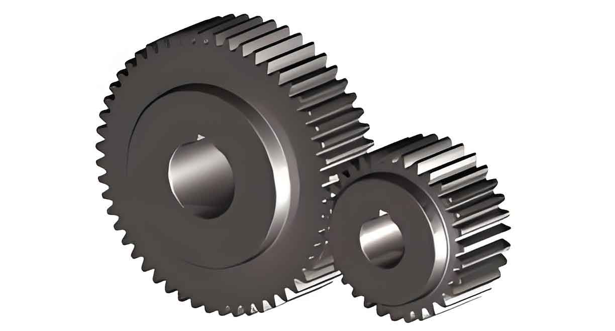
| Gear | Number of Teeth | Module (mm) | Pressure Angle (°) | Face Width (mm) |
|---|---|---|---|---|
| Driving Gear (1) | 43 | 3.2 | 20 | 52 |
| Driven Gear (2) | 39 | 3.2 | 20 | 52 |
From these basic geometric parameters, other dynamic parameters like mass, inertia, and average mesh stiffness are calculated. The non-dimensional parameters used in the state equations are set as follows: $F’_m=0.01$, $\zeta_{11}=\zeta_{22}=0.01$, $\zeta_{13}=\zeta_{23}=0.012$, $\zeta_{33}=0.05$, $F’_{b1}=0.1$, $F’_{b2}=0.2$. The fluctuating load is $F’_{aT}(t) = 0.05\omega^2 \sin(\omega t)$, where $\omega$ is the non-dimensional excitation frequency parameter. The static transmission error amplitude $\epsilon$ is 0.1. For the analysis focusing on gear backlash, the bearing clearance nonlinearity $f_{bi}$ is neglected to isolate the effect of the gear mesh backlash $b$.
To solve the system of nonlinear differential equations, I employ the fourth-order Runge-Kutta method (implemented via the ode45 function in a computational environment). Transient effects are discarded, and the steady-state response is analyzed. Bifurcation diagrams are constructed by plotting the local maxima of the torsional displacement $z_5$ against the varying control parameter (either $\omega$ or $b$). The corresponding Largest Lyapunov Exponent spectrum is calculated using the standard Wolf algorithm to quantify the nature of the attractor at each parameter value.
Results and Analysis: The Role of Excitation Frequency
First, I investigate the nonlinear dynamics of the spur gear system as the excitation frequency $\omega$ varies within the interval [2.2, 3.1], while keeping the backlash constant at $b=1.0$. The bifurcation diagram and the corresponding spectrum of the Largest Lyapunov Exponents (LLE) are presented below conceptually. The evolution is clear and demonstrates the powerful diagnostic capability of the LLE.
For low excitation frequencies in the range $2.2 < \omega < 2.35$, the spur gear system exhibits a stable single-period motion. The bifurcation diagram shows a single branch, and critically, the LLE is negative, confirming a periodic attractor. As $\omega$ increases beyond approximately 2.35, the system undergoes a sudden crisis, jumping directly into a chaotic regime. This is vividly captured by the LLE, which becomes positive in the range $2.35 \lesssim \omega \lesssim 2.54$. The bifurcation diagram in this region shows a broad, filled-in band of points, characteristic of chaos.
Upon further increase of $\omega$, the spur gear system exits chaos not through a reverse crisis, but through a period-doubling bifurcation cascade in reverse. Around $\omega \approx 2.54$, the LLE dips back below zero, and the bifurcation diagram collapses to a four-period orbit. This is a stable 4T motion. Continuing to $\omega \approx 2.645$, another reverse period-doubling occurs, leading to a stable two-period (2T) motion. Finally, for $\omega > 2.72$, the system undergoes a reverse period-doubling bifurcation back to a single-period (1T) motion, where it remains stable. Throughout the periodic windows (1T, 2T, 4T), the LLE remains strictly negative, providing quantitative validation of the periodic nature inferred from the bifurcation diagram.
To illustrate these states, let’s examine the time history, phase portrait, Poincaré map, and frequency spectrum for specific values of $\omega$:
- At $\omega = 2.3$ (Period-1): The time history is a perfect sinusoid. The phase portrait is a closed, single-loop curve. The Poincaré map (sampled at the excitation period) consists of a single isolated point. The frequency spectrum is dominated by a single peak at the excitation frequency.
- At $\omega = 2.52$ (Chaos): The time history is aperiodic and irregular. The phase portrait fills a bounded region of the phase space with a complex, fractal-like structure. The Poincaré map reveals a scatter of points forming a strange attractor. The frequency spectrum is broadband and continuous, indicating a wide range of excited frequencies.
- At $\omega = 2.57$ (Period-4): The time history shows a repeating pattern every four excitation periods. The phase portrait consists of four distinct loops. The Poincaré map contains four isolated points. The frequency spectrum shows a primary peak at $\omega/4$ and its harmonics.
- At $\omega = 3.0$ (Period-1): The characteristics are identical to those at $\omega=2.3$, confirming the return to a stable single-period motion for the spur gears at higher excitation frequencies in this parameter range.
Results and Analysis: The Role of Gear Backlash
Next, I fix the excitation frequency at $\omega = 2.3$ (a value originally in the periodic regime) and analyze the system’s behavior as the non-dimensional gear backlash $b$ varies within the small interval [0.06, 0.075]. This investigation is crucial for understanding how manufacturing tolerances or wear-induced clearance changes might destabilize a spur gear drive. The resulting bifurcation and LLE diagrams are highly revealing.
For very small backlash, $0.06 < b < 0.06125$, the system maintains a stable single-period motion, evidenced by a single branch in the bifurcation diagram and a negative LLE. However, a slight increase in backlash beyond $b \approx 0.06125$ triggers a dramatic change. The system experiences a crisis, plunging directly into a chaotic state. This transition is marked by the LLE jumping to a positive value for $0.06125 \lesssim b \lesssim 0.064$.
Interestingly, as I continue to increase the backlash for these spur gears, the system does not remain in sustained chaos. Instead, around $b \approx 0.064$, it undergoes a period-doubling bifurcation out of the chaotic sea, settling into a stable 4-period orbit. This is confirmed by the LLE becoming negative again in the range $0.064 < b < 0.07245$. The bifurcation diagram clearly shows four distinct branches.
The most complex behavior is observed for $b > 0.07245$. The system re-enters a chaotic state, but this chaos is now intermittently punctuated by very narrow periodic windows. This is known as intermittent or transient chaos. The LLE spectrum in this region reflects this instability: the exponent fluctuates around zero, frequently dipping negative (indicating brief periodic behavior) and spiking positive (indicating chaotic bursts). This regime is particularly dangerous from an engineering perspective, as the motion is unpredictable and can lead to intermittent high-impact forces within the spur gear mesh.
Dynamic response plots for selected backlash values further clarify these states:
- At $b = 0.059$ (Period-1): All indicators (time history, phase portrait, Poincaré map, spectrum) point to a clean, stable periodic motion, similar to the low-$\omega$ case.
- At $b = 0.063$ (Chaos): The plots show the classic signatures of chaos: aperiodic time trace, strange attractor in phase space, fractal Poincaré map, and broadband spectrum.
- At $b = 0.07$ (Period-4): The response is neatly period-4, with a four-loop phase portrait and a four-point Poincaré map.
- At $b = 0.073$ (Intermittent Chaos): The time history shows intervals of nearly periodic motion suddenly interrupted by irregular bursts. The Poincaré map shows a dense cluster of points (chaos) with some vague, incomplete structures suggesting the ghost of a periodic attractor.
Conclusion
Through this detailed nonlinear dynamics study of a three-degree-of-freedom spur gear model, I have successfully characterized the profound influence of key operational and design parameters on the system’s dynamic response. The use of the Largest Lyapunov Exponent as a primary diagnostic tool has been instrumental in providing unambiguous, quantitative evidence of dynamical transitions, particularly in distinguishing true chaos from complex periodic motion.
My analysis leads to two fundamental conclusions for spur gear design and operation:
- Excitation Frequency as a Control Parameter: The response of the spur gear system is highly sensitive to the meshing (excitation) frequency. For the given parameters, as frequency increases, the system transitions from stable period-1 motion into chaos via a boundary crisis, then exits chaos through an inverse period-doubling cascade (period-4 → period-2 → period-1), regaining stability at higher frequencies. The LLE trace perfectly mirrors this journey: negative → positive → negative. This map provides a clear guideline for avoiding chaotic operating speeds in spur gear applications.
- Backlash as a Critical Nonlinearity: Even minute changes in gear backlash can precipitate significant instability. Increasing backlash from a small value first drives the system from period-1 motion into chaos. Further increase can surprisingly lead to a period-doubling route out of chaos into a stable period-4 orbit. Ultimately, beyond a threshold, the system enters a region of unstable, intermittent chaos characterized by a wildly fluctuating LLE. This underscores the critical importance of tightly controlling and maintaining backlash within spur gear pairs to ensure predictable, stable dynamic performance and to prevent the onset of damaging chaotic impacts.
In summary, this research underscores the necessity of nonlinear analysis in the design of robust spur gear transmission systems. The bifurcation diagrams, when coupled with Lyapunov exponent analysis, offer a powerful framework for predicting complex dynamic behavior. The findings provide concrete theoretical benchmarks for selecting operational speeds and designing tolerance limits for backlash to keep spur gear systems within stable, predictable dynamical regimes, thereby enhancing their reliability and longevity in demanding mechatronic and intelligent manufacturing systems.