
In modern manufacturing and precision engineering, the accurate measurement of gear parameters is critical for ensuring performance, reliability, and interchangeability in mechanical systems. Among various gear types, the helical gear stands out due to its smooth operation, high load capacity, and reduced noise, making it widely used in automotive, aerospace, and industrial machinery. However, traditional contact-based measurement methods for helical gears are often time-consuming, prone to wear, and limited by probe accessibility, especially for parameters like helix angle and rotation direction. To address these challenges, I propose a non-contact, rapid detection approach leveraging machine vision techniques. This method enables comprehensive parameter extraction for helical gears, including addendum circle diameter, dedendum circle diameter, reference circle diameter, number of teeth, modulus, helix angle, and rotation direction. By integrating image processing, edge detection, least-squares fitting, and support vector machines (SVM), this system achieves high precision and stability, suitable for automated quality control and inline inspection.
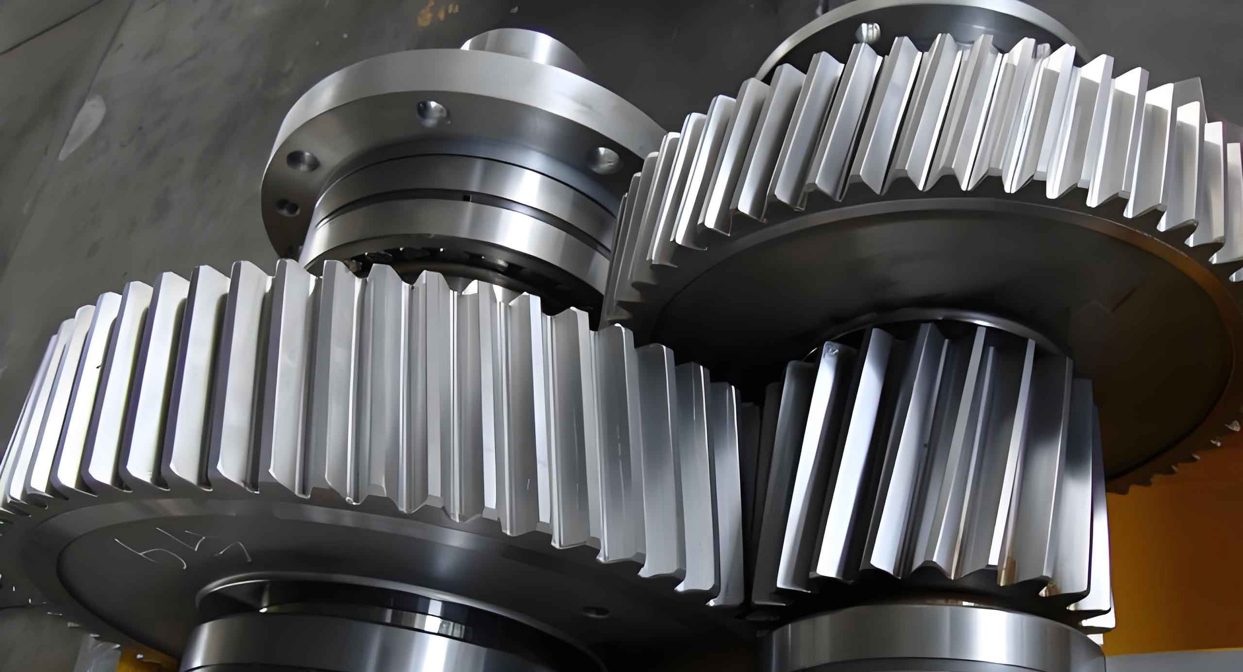
The core of this approach lies in capturing high-quality images of helical gears through a carefully designed vision system. A key component is the use of optimal lighting to enhance contrast and reduce noise. For instance, combining backlight and ring lighting illuminates the gear from different angles, highlighting edges and surface features. The following image illustrates a typical helical gear used in such setups, showcasing its intricate tooth geometry and spiral structure:
In my system, hardware includes a monochrome industrial camera (e.g., 2MP resolution), a telecentric lens to minimize distortion, and motion stages for positioning. The telecentric lens ensures consistent magnification regardless of object distance, critical for accurate dimensional measurements. After image acquisition, processing begins with preprocessing to improve clarity. I apply contrast enhancement using a formula that adjusts pixel gray values based on a mean filter and enhancement factor. For a given pixel with original gray value \(orig\), mean value \(mean\) from filtering, and factor \(Factor\), the new value \(res\) is computed as:
$$res = \text{round}((orig – mean) \times Factor + orig)$$
Through experimentation, I found that setting \(Factor = 2\) yields optimal enhancement, sharpening edges while suppressing background noise. This step is vital for subsequent segmentation and detection phases. Following preprocessing, threshold segmentation isolates the helical gear from the background. I use a global threshold \(T\), where pixels with gray values above \(T\) are set to 1 (object) and below to 0 (background), as defined by:
$$g(x,y) =
\begin{cases}
1, & \text{if } f(x,y) \geq T \\
0, & \text{if } f(x,y) < T
\end{cases}$$
This binarization results in a clear silhouette of the helical gear’s end face, facilitating edge extraction. For edge detection, I employ the Canny operator, which combines Gaussian smoothing, gradient calculation, non-maximum suppression, and hysteresis thresholding to achieve sub-pixel accuracy. Compared to other operators like Sobel or Roberts, Canny better handles noise and provides precise edge localization, essential for fitting circles and calculating parameters. The extracted contour includes both the outer addendum circle and inner dedendum circle edges, which are then used for geometric fitting.
To determine key parameters, I first locate the gear center by fitting a circle to the edge points using the least-squares method. For a set of points \((x_i, y_i)\), the circle equation is \(x^2 + y^2 + Ax + By + C = 0\), and minimizing the error \(E\) leads to:
$$E = \sum_{i=1}^{n} (x_i^2 + y_i^2 + A x_i + B y_i + C)^2$$
Solving the linear system derived from partial derivatives yields the center \((x_0, y_0) = (-A/2, -B/2)\) and radius. This allows fitting the minimum enclosing circle (addendum circle) and maximum inscribed circle (dedendum circle) to obtain diameters \(D_a\) and \(D_f\). The modulus \(m\) of the helical gear is then calculated using standard gear formulas. For helical gears, the addendum and dedendum diameters relate to modulus via:
$$D_a = D + 2h_a = m(z + 2h_a^*)$$
$$D_f = D – h_f = m(z – 2h_a^* – 2c^*)$$
where \(D\) is the reference diameter, \(z\) is the number of teeth, \(h_a^*\) is the addendum coefficient (typically 1), and \(c^*\) is the clearance coefficient (typically 0.25). Rearranging, the modulus is derived as:
$$m = \frac{D_a – D_f}{4h_a^* + 2c^*} = \frac{D_a – D_f}{4.5}$$
This value is compared against standard modulus tables to select the nearest standardized value. Common standard moduli for involute cylindrical gears are listed below:
| Standard Modulus (mm) |
|---|
| 0.1 |
| 0.12 |
| 0.15 |
| 0.2 |
| 0.25 |
| 0.3 |
| 0.4 |
| 0.5 |
| 0.6 |
| 0.8 |
| 1.0 |
| 1.25 |
| 1.5 |
| 2.0 |
| 2.5 |
| 3.0 |
| 4.0 |
| 5.0 |
| 6.0 |
| 8.0 |
| 10.0 |
| 12.0 |
| 16.0 |
| 20.0 |
| 25.0 |
| 32.0 |
| 40.0 |
| 50.0 |
The number of teeth \(z\) is detected by segmenting the gear end face image after morphological operations. I draw a region of interest (ROI) based on the reference circle, which is computed from the center and modulus, then count independent tooth regions. This process reliably yields the tooth count, crucial for verifying other parameters. For helical gears, the reference diameter \(D\) is linked to modulus and tooth count by \(D = m \times z\), allowing cross-validation of measurements.
Beyond basic geometric parameters, the rotation direction (handedness) of a helical gear—whether left-hand or right-hand—is essential for assembly and function. I classify this using a support vector machine (SVM), a supervised learning algorithm effective for binary classification with small datasets. The SVM finds an optimal hyperplane that maximizes the margin between two classes, defined for linear separation as minimizing \(\|w\|\) subject to constraints. For non-linear cases, kernel functions like radial basis function (RBF) map data to higher dimensions. Given a training set of gear side images binarized to highlight tooth inclination, I extract features such as edge gradients and spatial distributions. After testing various kernels, RBF achieves the highest accuracy (98%) in distinguishing left-hand from right-hand helical gears. The SVM decision function for a new sample \(x\) is:
$$f(x) = \text{sign}\left(\sum_{i=1}^{n} \alpha_i y_i K(x_i, x) + b\right)$$
where \(\alpha_i\) are Lagrange multipliers, \(y_i\) are labels, \(K\) is the kernel, and \(b\) is the bias. This automated classification eliminates subjective judgment and speeds up inspection.
Another critical parameter is the helix angle \(\beta\), which defines the tooth inclination relative to the gear axis. Traditional methods, like imprinting on paper or indirect calculation, are cumbersome. My vision-based method computes \(\beta\) from the gear side image by analyzing the tilt of the addendum surface. First, I locate the addendum region using template matching or edge detection. Then, I calculate the angle between the tooth trace and the horizontal axis, which corresponds to the addendum circle helix angle \(\beta_a\). The relationship between \(\beta_a\) and the reference circle helix angle \(\beta\) is derived from gear geometry:
$$\tan \beta_a = \frac{D_a}{D} \tan \beta$$
Rearranging, the reference helix angle is:
$$\beta = \arctan\left(\frac{D}{D_a} \tan \beta_a\right)$$
Here, \(D\) and \(D_a\) are known from earlier measurements, and \(\beta_a\) is obtained by fitting a line to the addendum edge points and computing its slope. This approach provides a direct, non-contact measurement of helix angle, adaptable to various helical gear sizes.
To validate the method, I conducted experiments on multiple standard helical gears with known specifications. The system was tested for accuracy, repeatability, and robustness under different lighting and positioning conditions. Below are tables summarizing detection results for key parameters. Table 1 shows addendum and dedendum diameter measurements for five helical gear samples, comparing detected values against actual values and calculating relative errors.
| Sample | Detected Addendum Diameter (mm) | Actual Addendum Diameter (mm) | Relative Error | Detected Dedendum Diameter (mm) | Actual Dedendum Diameter (mm) | Relative Error |
|---|---|---|---|---|---|---|
| 1 | 34.80 | 34.96 | 0.46% | 27.90 | 27.81 | 0.32% |
| 2 | 34.66 | 34.96 | 0.86% | 27.88 | 27.81 | 0.25% |
| 3 | 46.50 | 46.62 | 0.26% | 37.15 | 37.08 | 0.19% |
| 4 | 47.03 | 46.62 | 0.88% | 36.98 | 37.08 | 0.27% |
| 5 | 46.62 | 46.40 | 0.47% | 37.12 | 37.24 | 0.32% |
The average relative error for addendum diameter is 0.59% and for dedendum diameter is 0.27%, demonstrating high precision. Table 2 presents results for tooth count and modulus detection, which show perfect alignment with actual values, underscoring the reliability of the image processing pipeline.
| Sample | Detected Tooth Count | Actual Tooth Count | Detected Modulus (mm) | Actual Modulus (mm) |
|---|---|---|---|---|
| 1 | 20 | 20 | 1.5 | 1.5 |
| 2 | 20 | 20 | 1.5 | 1.5 |
| 3 | 20 | 20 | 2.0 | 2.0 |
| 4 | 20 | 20 | 2.0 | 2.0 |
| 5 | 20 | 20 | 2.0 | 2.0 |
For rotation direction and helix angle, Table 3 summarizes outcomes. The SVM classifier correctly identified all samples’ handedness, while helix angle measurements had an average relative error of 0.49%, well within acceptable limits for industrial applications.
| Sample | Detected Rotation Direction | Actual Rotation Direction | Detected Helix Angle \(\beta\) (°) | Actual Helix Angle \(\beta\) (°) | Relative Error |
|---|---|---|---|---|---|
| 1 | Left-hand | Left-hand | 19.28 | 19.31 | 0.16% |
| 2 | Left-hand | Left-hand | 19.47 | 19.31 | 0.82% |
| 3 | Right-hand | Right-hand | 19.22 | 19.31 | 0.46% |
| 4 | Right-hand | Right-hand | 11.99 | 12.08 | 0.75% |
| 5 | Right-hand | Right-hand | 12.11 | 12.08 | 0.25% |
The overall performance confirms that this machine vision approach is effective for helical gear parameter detection. It offers several advantages: non-contact operation preserves gear integrity, high-speed processing enables real-time inspection, and automation reduces labor costs. The integration of advanced algorithms like least-squares fitting and SVM enhances accuracy and adaptability to various helical gear designs. Potential improvements could involve deep learning for defect detection or 3D reconstruction for more complex gear geometries.
In conclusion, the proposed method provides a comprehensive solution for helical gear parameter measurement using machine vision. By combining image enhancement, edge detection, circle fitting, and machine learning, it achieves precise detection of diameters, tooth count, modulus, rotation direction, and helix angle. Experimental results validate its stability and accuracy, with errors typically below 1%. This system can be deployed in production lines for quality assurance, reducing reliance on manual inspection and facilitating Industry 4.0 initiatives. Future work may focus on extending the method to other gear types, such as bevel or worm gears, and optimizing hardware for even higher throughput. The versatility of machine vision continues to drive innovations in metrology, and helical gears represent a prime application area where these technologies can deliver significant value.