
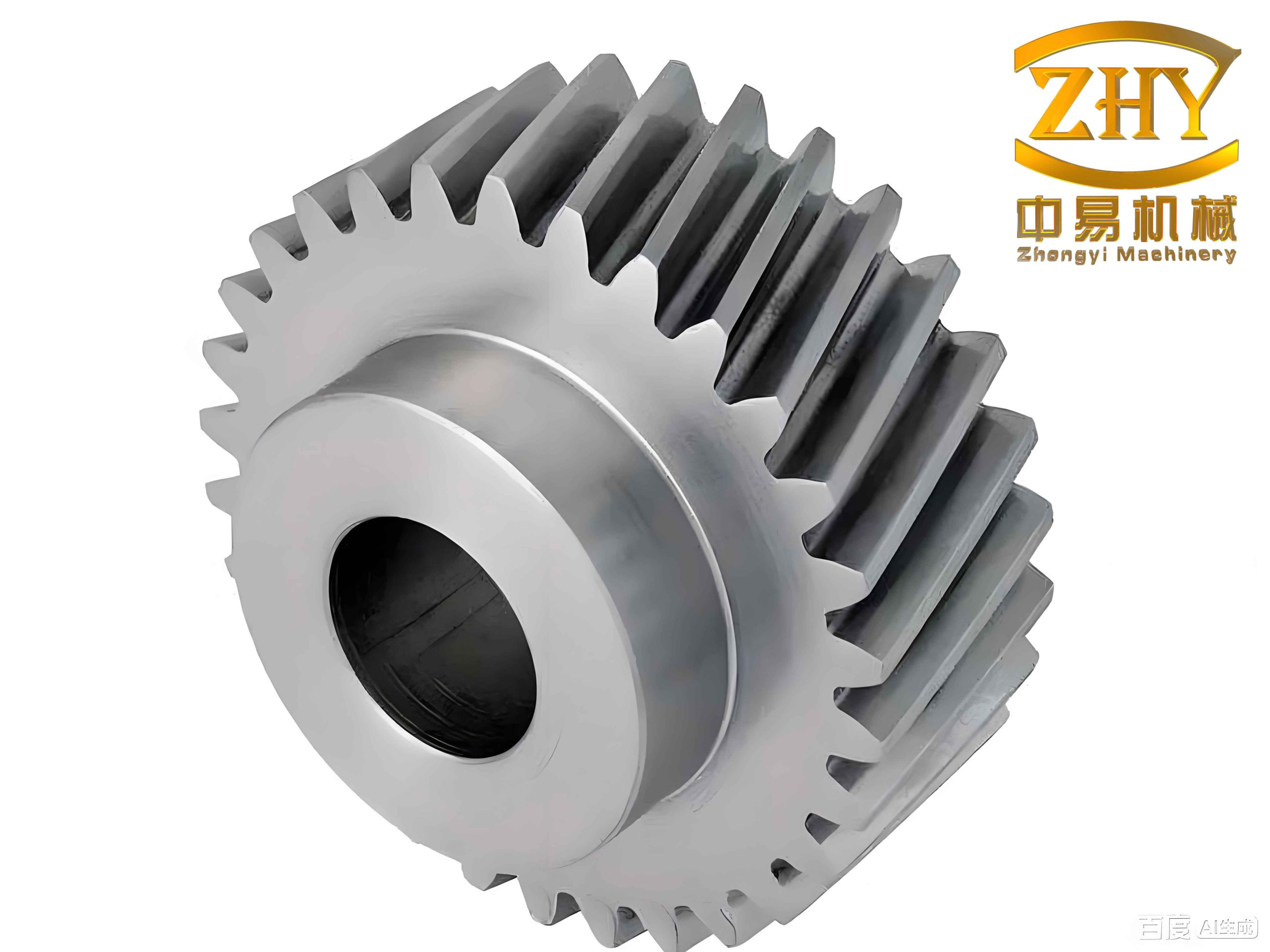
I have focused my research on the rapid, non-contact, and automated measurement of helical gear parameters. A helical gear is widely used in transmissions because it offers smoother motion, lower noise, and higher load capacity than a spur gear. However, the helical angle and the hand of the helix make the measurement problem more complex than that of a spur gear. Traditional contact instruments such as micrometers, height gauges, and universal angle rulers can reach high accuracy, but they are slow and sensitive to human operation. I therefore designed a multi-camera machine vision system that measures the face parameters and the side parameters of a helical gear in one station. The system estimates the addendum circle diameter, the dedendum circle diameter, the number of teeth, the hand of the helix, and the helical angle. My goal is to provide a practical method for on-line inspection of a helical gear in industrial production.
The main contribution of my work is the integration of several machine vision algorithms into a single helical gear measurement flow. I use a face camera for the end face of the helical gear and a side camera for the flank of the helical gear. The face camera measures the tooth count and the diameters of the addendum and dedendum circles. The side camera measures the hand of the helix and the helical angle. The two cameras share calibration data and pixel equivalence data. A graphical user interface allows preview and result display. I also introduce an edge continuation algorithm for broken tooth contours, a sub-pixel edge detection strategy for diameter measurement, a curvature-based curve fitting method for the helical angle, and a morphological structure-element counting method for the hand of the helix.
Measurement System Design
I built the measurement system as a compact station that can be inserted into a production line. The helical gear is supported by a shaft or a stepped cylinder. The face camera is mounted above the helical gear, and the side camera is mounted horizontally beside the helical gear. A ring light or a front light illuminates the end face, and a bar light or a partially masked flat light illuminates the side. Because a helical gear has a twisted tooth surface, a backlight cannot be used for side measurement. I therefore use front illumination for the side view, which increases the difficulty of edge extraction but is compatible with the real geometry of a helical gear.
I selected different lenses for different module ranges. For larger module helical gears, I use an ordinary industrial lens with a high-resolution CMOS sensor. For smaller module helical gears, I use a double telecentric lens with a smaller sensor. The double telecentric lens reduces perspective error and keeps the pixel equivalence almost constant within its working distance. The ordinary lens gives a larger field of view and a lower cost. The side camera uses a double telecentric lens when possible, because the helical angle is sensitive to perspective distortion. I also use a linear scale or a gauge block to determine the pixel equivalence before measurement.
| Camera position | Lens type | Typical use | Main advantage | Main limitation |
|---|---|---|---|---|
| Face | Ordinary industrial lens | Larger module helical gear | Large field of view and low cost | Perspective error away from the optical axis |
| Face | Double telecentric lens | Smaller module helical gear | Low distortion and stable pixel equivalence | Small field of view and higher cost |
| Side | Double telecentric lens | Helical angle and hand measurement | Reduced perspective error on the flank | Requires careful alignment with the gear axis |
I calibrated the ordinary camera with a chessboard target. I used multiple views and estimated the intrinsic matrix, the extrinsic matrix, and the distortion coefficients. For the telecentric camera, I used the calibration module of a machine vision software package. In both cases, I corrected radial and tangential distortion before parameter extraction. I also measured the tilt of the helical gear image so that the image coordinate system could be aligned with the world coordinate system. This step is important because the helical angle measurement depends on the direction of the gear axis.
Image Preprocessing
I first convert the color image to a grayscale image. This reduces the data volume and simplifies the subsequent calculations. I then apply a global low-illumination enhancement when the exposure time is very short. The enhancement improves the visual contrast, but I use it mainly for preview and debugging. For actual measurement, I rely on adaptive thresholding and edge detection rather than on a single global enhancement. I extract the region of interest by background subtraction. The background image is acquired before the helical gear enters the field of view. I subtract the background from the current image, binarize the result, remove small connected components, and compute the gray-level centroid. The centroid gives the approximate position of the helical gear. I trigger image acquisition when the centroid is close to the image center, which reduces lens distortion and perspective error.
I use Otsu thresholding for the low-illumination binarization step because it is fast and robust when the histogram has two main peaks. I compared Otsu with triangle thresholding and two local thresholding methods. The local methods amplified small brightness changes caused by reflection, while Otsu ignored those changes. The Otsu method required about 0.14 ms for a typical region of interest, which is acceptable for on-line measurement.
| Binarization method | Type | Observed behavior on my images | Speed |
|---|---|---|---|
| Otsu | Global adaptive | Good separation of the helical gear from the background | Fast |
| Triangle | Global adaptive | Acceptable for single-peak histograms, less stable here | Fast |
| Niblack | Local adaptive | Sensitive to background reflection | Moderate |
| Wellner | Local adaptive | Too sensitive to small illumination changes | Moderate |
The pixel equivalence is the physical size represented by one pixel. For a telecentric lens, the pixel equivalence is nearly constant within the working distance. For an ordinary lens, the pixel equivalence changes with the object distance. I use a gauge block with a known length to determine the pixel equivalence. I measure the same edge in two positions with different heights and solve for the true object distance. Let \(pix_s\) be the pixel equivalence when the block stands vertically, and let \(pix_l\) be the pixel equivalence when the block lies flat. If the height difference is \(\Delta h\), I can write
$$ \frac{pix_s}{pix_l} = \frac{w + \Delta h}{w} $$
where \(w\) is the object distance for the standing block. I solve for \(w\), and then I compute the pixel equivalence for other heights. For the telecentric lens, I use the gauge block directly and do not apply this correction. The pixel equivalence values I obtained are summarized below.
| Lens type | Measured height | Pixel equivalence | Use case |
|---|---|---|---|
| Double telecentric | 9 mm | 24.13 μm | Small module helical gear |
| Ordinary lens 1 | 20 mm | 13.58 μm | Medium module helical gear with short working distance |
| Ordinary lens 2 | 20 mm | 38.02 μm | Large module helical gear with long working distance |
Edge Extraction for Helical Gear Images
Edge extraction is the bridge between image preprocessing and parameter extraction. I treat the end face and the side face separately because their imaging characteristics are different. The end face of a helical gear is mostly flat and has a strong contrast with the background. The side face has a twisted surface, uneven illumination, and many surface defects. A single edge detector with fixed thresholds cannot handle both cases well. I therefore designed two edge extraction flows.
End Face Edge Extraction
For the end face image, I apply Gaussian filtering before edge detection. The Gaussian filter suppresses fine machining marks and dust while preserving the main tooth contour. I then use an adaptive Canny detector with thresholds derived from the Otsu method. The Otsu method finds a threshold that maximizes the between-class variance. I use this threshold to set the high and low thresholds of the Canny detector. The resulting edges are thin and well localized. However, metal chips or surface defects can break the contour. I therefore apply an edge continuation algorithm. I first thin the edge image, find endpoints, and connect endpoint pairs that are within a distance threshold. This step closes small gaps and makes the outer contour a single connected component.
| Step | Algorithm | Purpose | Observed effect |
|---|---|---|---|
| Filtering | Gaussian filter | Suppress scratches and dust | Reduced false edges |
| Edge detection | Otsu adaptive Canny | Extract tooth contour | Thin and continuous in most regions |
| Edge continuation | Endpoint detection and DDA line drawing | Close contour gaps | Improved hole filling and contour tracking |
Side Face Edge Extraction
For the side face image, the main problem is uneven illumination. The tooth flank of a helical gear is curved, and the brightness changes from the left side to the right side. I compared several filtering methods, including discrete cosine transform denoising, high dynamic range synthesis, Gaussian filtering, vignetting correction, homomorphic filtering, high-pass contrast preservation, edge-preserving sharpening, and low-pass filtering. The vignetting correction method gave the best balance between speed and edge quality. Its principle is to minimize the entropy of the image while correcting the dark corners. I then apply the Canny detector with a Gaussian filter. The resulting edge image still contains redundant edges from surface scratches and highlights. To isolate the true tooth line, I use a morphological slope screening method.
The morphological slope screening uses structure elements that represent the expected slope of the tooth line. I build several small binary kernels. One kernel represents a positive slope, another represents a negative slope, and another represents a horizontal line. I scan the edge image and count the number of matches. The hand of the helix is determined by comparing the counts. I then remove horizontal and vertical structures that do not belong to the tooth line. This step is fast and works well even when the illumination is nonuniform.
| Filtering method | Edge continuity | Noise suppression | Speed | Suitability for helical gear side view |
|---|---|---|---|---|
| Discrete cosine transform denoising | Moderate | Moderate | Fast | Limited |
| High dynamic range synthesis | Good | Good | Slow | Not suitable for on-line use |
| Gaussian filtering | Good | Moderate | Fast | Useful as a pre-filter |
| Vignetting correction | Good | Good | Fast | Best overall in my tests |
| Homomorphic filtering | Moderate | Good | Moderate | Acceptable but hard to tune |
| Edge-preserving sharpening | Moderate | Low | Fast | Amplifies surface defects |
Face Parameter Extraction of a Helical Gear
The face parameters of a helical gear include the number of teeth \(z\), the addendum circle diameter \(d_a\), the dedendum circle diameter \(d_f\), the pitch circle diameter \(d\), the base circle diameter \(d_b\), and the module \(m\). I measure the tooth count and the two diameters directly. I then derive the pitch circle diameter and the base circle diameter using standard relationships. For a standard helical gear, the following relations hold:
$$ d = m z $$
$$ d_a = d + 2m $$
$$ d_f = d – 2.5m $$
$$ d_b = d \cos \alpha $$
where \(\alpha\) is the pressure angle at the pitch circle. In my experiments, \(\alpha\) is 20 degrees for the standard helical gear. I use the measured dedendum circle diameter as the primary quantity for deriving the pitch circle diameter, because the addendum of a helical gear is often chamfered or polished after hobbing. The dedendum circle is less affected by finishing operations.
Tooth Count Measurement
I measure the tooth count by connected component analysis. First, I compute the approximate addendum circle diameter and dedendum circle diameter by pixel-level edge detection. I then create a circular mask whose diameter is the average of the two diameters. I multiply the mask by the binarized image. This isolates the teeth from the inner hole and the keyway. I then count the connected components after a small erosion. The number of connected components is the number of teeth. I also compute the centroid of each connected component. These centroids are used later to classify sub-pixel edge points. The tooth count measurement is robust and is not affected by the helical angle.
| Tooth count method | Principle | Robustness | Speed | Use in my system |
|---|---|---|---|---|
| Intersection method | Intersect a circle with the tooth edge and count intersections | Moderate | Fast | Used as a check |
| Connected component method | Mask the tooth region and count components | High | Fast | Primary method |
| Radial unfolding method | Unwrap the edge and count periodic peaks | Moderate | Moderate | Not used |
Initial Diameter Measurement
I use the outer contour of the helical gear to estimate the addendum circle diameter. After edge continuation and hole filling, the outer contour is a single closed boundary. I compute the geometric center by averaging the coordinates of the contour points. I then compute the distance from each contour point to the center. For the addendum circle, the maximum distances occur on the tooth tips. I use a minimum enclosing circle algorithm to obtain an initial value. For the dedendum circle, the minimum distances occur at the tooth roots. I use a maximum inscribed circle algorithm to obtain an initial value. These initial values are accurate enough to build the circular mask for tooth counting.
The geometric center is computed as follows. Let the contour points be \((x_i, y_i)\), and let \(N\) be the number of contour points. The center \((x_c, y_c)\) is
$$ x_c = \frac{1}{N} \sum_{i=1}^{N} x_i $$
$$ y_c = \frac{1}{N} \sum_{i=1}^{N} y_i $$
The initial addendum circle diameter \(d_{a0}\) is
$$ d_{a0} = \frac{2}{N} \sum_{i=1}^{N} \sqrt{(x_i – x_c)^2 + (y_i – y_c)^2} $$
This estimate is not the final value because the contour includes both tooth tips and tooth roots. However, it is sufficient for the mask and for the tooth count.
Sub-Pixel Edge Detection for Diameter Measurement
To improve the diameter accuracy, I use a sub-pixel edge detector based on partial area effect. The detector assumes that the edge crosses a pixel and divides the pixel into two regions with intensities \(A\) and \(B\). The observed pixel value is a weighted average of the two intensities. For a pixel \((i, j)\), the model is
$$ I_{i,j} = B + \frac{A – B}{h^2} P_{i,j} $$
where \(h\) is the pixel side length, and \(P_{i,j}\) is the area of the lower-intensity region inside the pixel. I use a \(5 \times 3\) window and solve for the edge parameters. The edge is represented by \(y = a + b x\) inside the pixel. The coefficients are obtained from the sums of the left, middle, and right columns. The sub-pixel edge point is located at \((0, a)\) in the pixel coordinate system. The normal vector of the edge is
$$ \mathbf{n} = \frac{[A – B]}{\sqrt{1 + b^2}} \begin{bmatrix} -b \\ 1 \end{bmatrix} $$
This method is fast and accurate. It works well when the edge is not perfectly straight because the window is small. I apply it to the original gray image, not to the binary image. The sub-pixel points are then classified by their angular position relative to the gear center. I use the centroids of the connected tooth components to define angular sectors. Each sector contains one tooth. For the addendum circle, I rotate the sectors by half a tooth pitch so that each sector contains a complete tooth tip. I select the point with the maximum radial distance in each sector. For the dedendum circle, I select the point with the minimum radial distance in each sector. I then fit a circle to the selected points using least squares.
Let the selected points be \((x_k, y_k)\) for \(k = 1, 2, \ldots, M\). The least squares circle fit minimizes
$$ \sum_{k=1}^{M} \left( \sqrt{(x_k – x_c)^2 + (y_k – y_c)^2} – R \right)^2 $$
I solve this nonlinear problem by linearization or by an iterative method. After the first fit, I compute the residuals and remove outliers using the \(3\sigma\) rule. I then perform a second fit. This improves the robustness against chips and scratches. The final diameters are \(d_a = 2R_a\) and \(d_f = 2R_f\).
| Helical gear number | Module (mm) | Tooth number | Design addendum diameter (mm) | Measured addendum diameter (mm) | Absolute error (mm) | Relative error (%) |
|---|---|---|---|---|---|---|
| 1# | 1.5 | 26 | 58.15 | 58.1215 | 0.0285 | 0.049 |
| 2# | 1.5 | 26 | 58.15 | 58.1328 | 0.0172 | 0.030 |
| 3# | 1.25 | 25 | 35.66 | 35.6556 | 0.0044 | 0.012 |
| 4# | 1.25 | 25 | 35.66 | 35.6487 | 0.0113 | 0.032 |
| 5# | 1.5 | 26 | 58.15 | 58.1661 | 0.0161 | 0.028 |
| Helical gear number | Module (mm) | Tooth number | Design dedendum diameter (mm) | Measured dedendum diameter (mm) | Absolute error (mm) | Relative error (%) |
|---|---|---|---|---|---|---|
| 1# | 1.5 | 26 | 51.4 | 51.3814 | 0.0186 | 0.036 |
| 2# | 1.5 | 26 | 51.4 | 51.3845 | 0.0155 | 0.030 |
| 3# | 1.25 | 25 | 30.0035 | 29.9941 | 0.0094 | 0.031 |
| 4# | 1.25 | 25 | 30.0035 | 29.9913 | 0.0122 | 0.041 |
| 5# | 1.5 | 26 | 51.4 | 51.4258 | 0.0258 | 0.050 |
The average absolute error of the addendum circle diameter is about 15.5 μm, and the average relative error is about 0.030%. The average absolute error of the dedendum circle diameter is about 16.3 μm, and the average relative error is about 0.038%. These values are close to the precision of a vernier caliper. The tooth count measurement is 100% correct in my experiments. The measurement time for the face parameters is less than 0.5 s.
Side Parameter Extraction of a Helical Gear
The side parameters of a helical gear are the hand of the helix and the helical angle. The hand determines whether the helical gear is left-handed or right-handed. The helical angle determines the transmission characteristics. I measure both parameters from the side image. The side image is more difficult than the face image because the tooth line is a space curve projected onto a plane. I model the tooth line mathematically and then fit the projected curve.
Mathematical Model of the Helical Gear Tooth Line
Let the helical gear axis be the \(z\)-axis in a three-dimensional coordinate system. The helix on the pitch cylinder can be parameterized as
$$ x = r \cos\left(\theta_0 + \frac{2\pi(n-1)}{z} + \theta\right) $$
$$ y = r \sin\left(\theta_0 + \frac{2\pi(n-1)}{z} + \theta\right) $$
$$ z = \frac{r \theta}{\tan \beta} $$
where \(r\) is the radius of the cylinder, \(z\) is the number of teeth, \(\beta\) is the helical angle, \(\theta_0\) is the initial angular position, and \(n\) is the tooth index. The sign of \(\beta\) indicates the hand of the helix. For a left-handed helical gear, the tooth line rotates in one direction as \(z\) increases; for a right-handed helical gear, it rotates in the opposite direction. The projection of the helix onto the \(xoz\) plane is not a straight line. However, the central tooth line is close to a straight line when the helical angle is small. For large helical angles, the curvature is significant, and a straight-line approximation causes a systematic error.
I derived the projection function for the visible part of the tooth line. If the camera observes the front of the helical gear, the visible range is \(0 \lt \theta_0 + 2\pi(n-1)/z + \theta \lt \pi\). The relation between \(x\) and \(z\) for one tooth line can be written as
$$ z – z_0 = \frac{x – x_0}{\tan \beta} \pm r \sqrt{1 – \left(\frac{x – x_0}{r}\right)^2} $$
This expression shows that the projected curve is unique for a given helical angle. I simulated the projected curve for different helical angles and confirmed that no two angles produce the same shape. This uniqueness is the theoretical basis of my side measurement method.
Hand of the Helix
I determine the hand of the helix by counting morphological structure elements in the edge image. A left-handed helical gear and a right-handed helical gear produce different dominant slopes in the side image. I define a positive-slope kernel and a negative-slope kernel. I also define a horizontal kernel to detect horizontal lines that do not belong to the tooth line. I scan the edge image and count the number of matches for each kernel. The counts differ greatly between left-handed and right-handed helical gears. I use the ratio of the two counts as a decision rule. The method is fast and robust even when the image is overexposed.
| Helical gear number | Module (mm) | Tooth number | Helical angle (degrees) | Hand | Positive-slope count | Negative-slope count |
|---|---|---|---|---|---|---|
| Z-1# | 1.5 | 26 | 45 | Right | 28861 | 11946 |
| Z-2# | 1.5 | 22 | 19 | Left | 1569 | 2637 |
| Z-3# | 2 | 30 | 19 | Left | 2270 | 3988 |
| Z-4# | 1.5 | 30 | 19 | Left | 443 | 1004 |
| Z-5# | 1.25 | 25 | 0 | Spur gear | 934 | 3242 |
The structure-element method runs in about 27 ms on a region of interest of \(781 \times 1558\) pixels. It does not require a separate training step. It is therefore suitable for on-line hand detection of a helical gear.
Helical Angle Measurement by Curve Fitting
After I determine the hand, I extract the tooth line edges. I remove short connected components and use the morphological slope screening to isolate the central tooth lines. I then transform the image coordinates into a coordinate system whose \(y\)-axis is parallel to the gear axis and whose \(x\)-axis is the end face line. I correct the tilt of the helical gear image using the axis or the end face contour. The transformation is
$$ x_{real1} = y_{img} – x_0 $$
$$ y_{real1} = x_{img} – y_0 $$
$$ x_{real2} = x_{real1} \cos \theta_{rotate} – y_{real1} \sin \theta_{rotate} + x_0 $$
$$ y_{real2} = x_{real1} \sin \theta_{rotate} + y_{real1} \cos \theta_{rotate} + y_0 $$
where \((x_0, y_0)\) is the gear center in the image coordinate system, and \(\theta_{rotate}\) is the tilt angle. I fit the visible edge points of one central tooth line to the projected helix model. I use a numerical solver to minimize the variance between the measured points and the model. I vary the helical angle in small steps and select the angle that gives the minimum variance. The step size I use is \(0.00029\) rad. The fit is repeated for several tooth lines, and the median value is taken as the final helical angle. This reduces the influence of local defects.
The relation between the addendum helical angle \(\beta_a\) and the pitch helical angle \(\beta\) is
$$ \tan \beta_a = \frac{\pi d_a}{P} $$
$$ \tan \beta = \frac{\pi d}{P} $$
where \(P\) is the lead of the helix. Therefore,
$$ \beta = \arctan\left( \frac{d}{d_a} \tan \beta_a \right) $$
I measure \(\beta_a\) from the tooth tip curve and convert it to the pitch helical angle. This conversion is important because the side image shows the tooth tip more clearly than the pitch line in many cases. The conversion also allows me to use the face measurement of \(d_a\) and \(d\) as inputs. The final helical angle is reported at the pitch circle.
| Helical gear number | Design helical angle (degrees) | Measured helical angle (degrees) | Absolute error (arc minutes) | Absolute error (degrees) | Relative error (%) |
|---|---|---|---|---|---|
| 1# | 45.00 | 45.1057 | 6.34 | 0.1057 | 0.23 |
| 2# | 45.00 | 45.1255 | 7.53 | 0.1255 | 0.28 |
| 3# | 19.524 | 19.4510 | 4.38 | 0.0730 | 0.37 |
| 4# | 19.524 | 19.6172 | 5.59 | 0.0932 | 0.48 |
| 5# | 45.00 | 44.8710 | 7.74 | 0.1290 | 0.29 |
The average absolute error of the helical angle is about 6.3 arc minutes, and the average relative error is about 0.33%. The measurement precision is close to that of a universal angle ruler. The total measurement time is about 1 s. This is much faster than manual measurement and is suitable for on-line inspection of a helical gear.
Error Analysis
I analyzed the error sources of the face parameter measurement and the side parameter measurement. For the face parameters, the main error sources are pixel equivalence error, surface defects, and eccentricity. The pixel equivalence error has a linear effect on the diameter measurement. A relative error of 0.1% in the pixel equivalence produces a relative error of 0.1% in the measured diameter. Surface defects such as chips, scratches, and dust can create false edge points. The least squares circle fit with the \(3\sigma\) rule reduces this effect. Eccentricity occurs when the camera optical axis is not aligned with the gear center. The sub-pixel feature point selection is sensitive to eccentricity because the angular sectors are defined by the gear center. I reduce this error by triggering image acquisition when the helical gear is near the image center.
For the helical angle measurement, the main error sources are assembly error, tilt correction error, surface defects, and chamfering. Assembly error includes the tilt of the side camera and the misalignment of the gear axis. Tilt correction error arises because I correct the image tilt using the axis or the end face contour. If the gear axis is not perfectly straight, the correction is incomplete. Surface defects such as scratches and stains can break the tooth line edge. I remove short edges and use the median of multiple tooth lines to reduce this error. Chamfering is a common finishing operation. The chamfer removes the sharp edge at the tooth tip, so the tooth tip curve is not exactly on the addendum cylinder. This introduces a small bias in the helical angle. I measure the helical gear before chamfering when possible. When chamfering is unavoidable, I use the central part of the tooth flank for fitting.
| Parameter | Main error source | Mitigation method | Observed residual error |
|---|---|---|---|
| Addendum diameter | Pixel equivalence, chamfer, eccentricity | Gauge block calibration, sub-pixel edge detection, center triggering | About 15.5 μm |
| Dedendum diameter | Surface defects, chips, pixel equivalence | Masking, \(3\sigma\) outlier removal, least squares fit | About 16.3 μm |
| Tooth count | Broken contour, small connected components | Edge continuation, erosion, connected component counting | No error in my tests |
| Hand of helix | Overexposure, noise | Structure-element counting, Gaussian pre-filter | No error in my tests |
| Helical angle | Assembly, tilt, chamfer, surface defects | Telecentric lens, tilt correction, curve fitting, median of lines | About 6.3 arc minutes |
Experimental Results and Discussion
I tested the system on five helical gears. The modules are 1.25 mm and 1.5 mm. The tooth numbers are 25 and 26. The helical angles are 19.524 degrees and 45 degrees. The hands are left and right. The design values were verified with a micrometer and a universal angle ruler. The measurement results are summarized in the tables above.
The face parameter measurement is accurate enough for production screening. The addendum and dedendum diameter errors are below 0.03 mm. This is comparable to a vernier caliper and is sufficient for sorting a helical gear into tolerance classes. The tooth count is exact. The measurement speed is limited mainly by image acquisition and edge detection. The whole face measurement takes less than 0.5 s.
The side parameter measurement is more challenging. The helical angle error is about 0.1 degree for a 45-degree helical gear and about 0.08 degree for a 19.5-degree helical gear. The error is larger for the 45-degree helical gear because the projected curve is more curved and the edge extraction is more difficult. The hand detection is exact in all tests. The side measurement takes about 0.5 s. The total system time is about 1 s per helical gear. This is fast enough for on-line inspection.
I compared my method with a straight-line approximation method. The straight-line method assumes that the central tooth line is a straight line. This assumption is acceptable for small helical angles and thin gears, but it causes a systematic error for large helical angles. In my test with a 45-degree helical gear, the straight-line method gave a relative error of about 2% to 3%. My curve fitting method reduced the relative error to about 0.3%. The improvement is significant for large helical angles.
| Method | Helical angle error for 45 degrees | Helical angle error for 19.5 degrees | Measurement time |
|---|---|---|---|
| Straight-line approximation | About 2% to 3% | About 0.5% to 1% | Fast |
| My curve fitting method | About 0.23% to 0.29% | About 0.37% to 0.48% | About 1 s |
| Universal angle ruler | About 0.1% to 0.2% | About 0.1% to 0.2% | Many seconds |
Industrial Application Scenarios
I expect the system to be used in several industrial scenarios. The first scenario is the inspection and classification of a helical gear semi-finished product. After hobbing, the helical gear still has machining allowance. The system measures the addendum circle, dedendum circle, tooth count, hand, and helical angle. If the helical gear is within tolerance, it is passed to the next process. If it is undersized, it is marked as scrap. If it is oversized, it is returned for further machining. A robot or a mechanical gate can sort the helical gear. The measurement data can be stored in a database for quality statistics. The statistics can help engineers improve the manufacturing process.
The second scenario is the measurement of a small-module helical gear. For a helical gear with an addendum circle diameter less than 10 mm, contact measurement is difficult because the probe may not fit into the tooth space. My machine vision method is non-contact and can measure such a helical gear easily. Small-module helical gears are common in drones, toy cars, and robotic vacuum cleaners. The third scenario is the measurement of other workpieces. The same system can be adapted to measure a spur gear or a shaft by changing the parameter extraction module. The hardware and the calibration flow remain the same.
Conclusion
I designed and tested a multi-camera machine vision system for helical gear parameter measurement. The system measures the addendum circle diameter, the dedendum circle diameter, the tooth count, the hand of the helix, and the helical angle. The face camera uses Gaussian filtering, Otsu adaptive Canny edge detection, edge continuation, connected component analysis, sub-pixel edge detection, and least squares circle fitting. The side camera uses vignetting correction, Canny edge detection, morphological slope screening, structure-element counting, and curve fitting. The two cameras are calibrated together, and the pixel equivalence is determined with a gauge block.
My experiments show that the addendum circle diameter error is about 15.5 μm, the dedendum circle diameter error is about 16.3 μm, and the helical angle error is about 6.3 arc minutes. The tooth count and the hand of the helix are measured without error in my tests. The total measurement time is about 1 s. The precision is close to a vernier caliper for the face parameters and close to a universal angle ruler for the helical angle. The method is suitable for on-line inspection of a helical gear.
In future work, I plan to improve the adaptivity of the filtering and edge detection parameters. I also plan to optimize the curve fitting algorithm to reduce the influence of outliers. Finally, I plan to implement the algorithm in a cross-platform application and test it on a real production line. I believe that machine vision will continue to play an important role in the measurement of a helical gear and other precision components.