
In my extensive work on mechanical power transmission systems, the analysis of spur gear contacts stands as a fundamental yet complex challenge. The spur gear, with its straightforward design of straight teeth parallel to the axis of rotation, is ubiquitous in machinery ranging from simple devices to complex industrial equipment like mining excavators. Its performance under dynamic loading conditions is paramount for system reliability. While analytical methods like the Hertzian contact theory provide a foundation, they often fall short in capturing the intricate, transient, and non-linear phenomena occurring during the meshing cycle of a spur gear pair, especially under heavy or impact loads. This is where explicit finite element analysis (FEA), particularly using a solver like LS-DYNA, becomes an indispensable tool in my engineering arsenal. It allows me to simulate the true dynamic contact behavior, providing insights into stress concentrations, deformation patterns, and potential failure modes that are otherwise difficult or impossible to obtain.
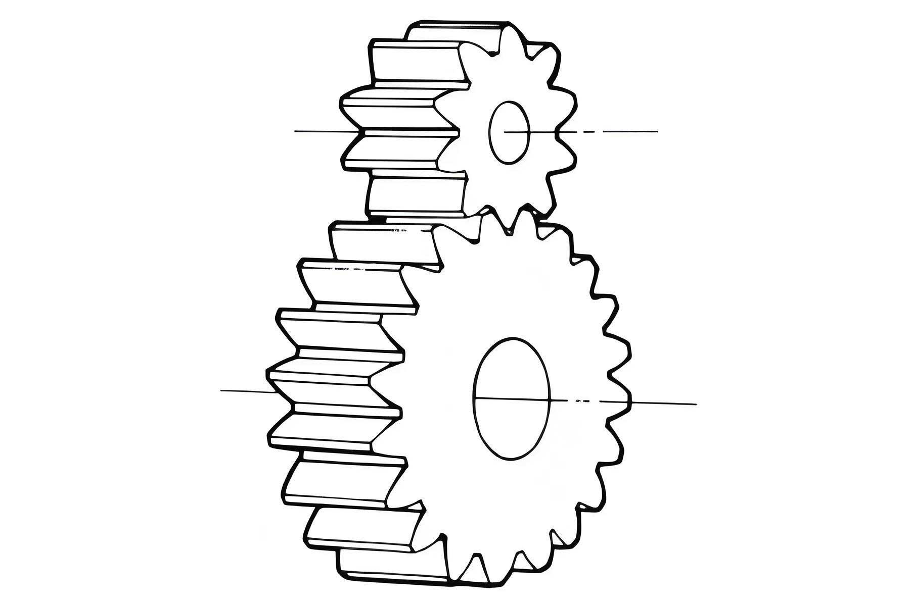
The core objective of my simulations is to accurately predict the contact stress evolution on the teeth flanks of a spur gear. The maximum contact stress is a critical parameter for assessing pitting resistance and contact fatigue life. The basic Hertzian contact stress for two parallel cylinders, which approximates the contact between two spur gear teeth, is given by:
$$ \sigma_H = \sqrt{\frac{F E_{eq}}{\pi \rho_{eq} L}} $$
where \( F \) is the normal load per unit face width \( L \), \( E_{eq} \) is the equivalent Young’s modulus, and \( \rho_{eq} \) is the equivalent radius of curvature at the contact point. However, this equation assumes static, smooth, and perfectly elastic contact. A dynamic simulation of a spur gear must account for time-varying load sharing, sliding and rolling friction, geometric transitions from single to double pair contact, and material plasticity. My workflow for achieving this with LS-DYNA involves a meticulous sequence of steps, each with its own set of critical decisions and potential pitfalls.
Geometry and Meshing: The Foundation of Accuracy
My journey begins not within the FEA environment, but in a dedicated parametric CAD software. I create a precise, three-dimensional model of the spur gear. I have found that for dynamic contact analysis, it is crucial to model the exact involute tooth profile. Small features like fillets at the tooth root are essential as they are high-stress regions; however, excessively small chamfers or radii can cause meshing failures later. I assemble the gear pair (or a gear train) with the correct center distance. For a typical two-gear simulation, I often model the driven gear as a flexible body (the focus of my analysis) and the driver as a rigid body to reduce computational cost, though both can be flexible for a fully coupled analysis.
Importing this geometry into the ANSYS pre-processor for LS-DYNA is straightforward via standard data exchange formats. The first and perhaps most impactful decision is the choice of element type. For a spur gear contact simulation, I primarily use two element types, as summarized in the table below:
| Element Type | LS-DYNA Name | Key Application in Spur Gear Analysis | Critical Settings |
|---|---|---|---|
| 8-Node Hexahedral Solid | SOLID164 | Main element for modeling the bulk material of the flexible spur gear teeth and body. It is well-suited for large deformation and contact. | Default formulation (usually constant stress). Hourglass control must be activated (e.g., Flanagan-Belytschko stiffness form) with a carefully chosen coefficient to prevent zero-energy modes without making the model too stiff. |
| 4-Node Shell | SHELL163 | Used to create a thin layer on the inner bore surface of the flexible spur gear. This is the key to applying rotational boundary conditions (velocities/torques) to the flexible component. | Real constants define thickness. For a pure kinematic constraint, I set a minimal, uniform thickness (e.g., 0.1 mm). The number of through-thickness integration points (NIP) is typically set to 2 or 3. |
Meshing is an art. I apply a fine, structured hex-dominant mesh in the contact region of the spur gear teeth to capture the high stress gradients accurately. The root fillet and the flank near the pitch line require particular attention. The rest of the gear body can have a coarser mesh. A common mistake is over-refining the entire model, which leads to prohibitively small time steps and excessive solve times. I use a bias function to gradually transition from fine elements on the teeth to coarser elements in the hub. The target element size on the tooth flank is often dictated by the expected size of the contact patch. As a rule of thumb, I aim for at least 3-5 elements across the minor axis of the elliptical contact area. The time step in an explicit analysis is governed by the Courant condition:
$$ \Delta t_{stable} = \frac{l_{min}}{c_d} $$
where \( l_{min} \) is the smallest element dimension in the model and \( c_d \) is the dilatational wave speed of the material \( \left( c_d = \sqrt{\frac{E}{\rho}} \right) \). Therefore, one tiny element dictates the pace for the entire simulation.
Material, Contacts, and Loading: Defining the Physics
For a spur gear made of steel, I typically use a bilinear isotropic hardening material model (*MAT_PIECEWISE_LINEAR_PLASTICITY in LS-DYNA). This model requires density \( \rho \), Young’s modulus \( E \), Poisson’s ratio \( \nu \), yield stress \( \sigma_y \), and tangent modulus \( E_t \). A critical pitfall here is unit consistency. Since I often define geometry in mm, I must use consistent units: Tonne (for mass), mm, and second (T-mm-s). In this system, density is in \( \text{Tonne/mm}^3 \) (e.g., steel density is \( 7.85 \times 10^{-9} \)), pressure/stress is in MPa (\( \text{N/mm}^2 \)), and energy is in mJ. Getting this wrong is a prime cause of nonsensical results or simulation failure.
| Material Property | Symbol | Typical Value for Steel | Unit (T-mm-s) |
|---|---|---|---|
| Density | \( \rho \) | \( 7.85 \times 10^{-9} \) | \( \text{Tonne/mm}^3 \) |
| Young’s Modulus | \( E \) | \( 2.10 \times 10^5 \) | MPa |
| Poisson’s Ratio | \( \nu \) | 0.3 | – |
| Yield Stress | \( \sigma_y \) | 450 – 1200 | MPa |
| Tangent Modulus | \( E_t \) | \( \sim 0.01E \) to \( 0.1E \) | MPa |
The heart of a spur gear simulation is the contact definition. I almost exclusively use the automatic surface-to-surface contact (*CONTACT_AUTOMATIC_SURFACE_TO_SURFACE). For a pair of gears, I define two separate contact interfaces: one between Gear 1 and Gear 2, and another if a third gear is present. The beauty of the “automatic” type is that it does not require pre-defining slave and master surfaces; the algorithm determines the interaction dynamically, which is ideal for the complex, changing contact conditions in a meshing spur gear set. Key parameters I adjust are the static (\( \mu_s \)) and dynamic (\( \mu_d \)) friction coefficients, which I often set between 0.05 and 0.15 for lubricated steel contacts. The contact stiffness is another critical parameter; I typically let LS-DYNA determine it automatically based on the bulk modulus of the contacting materials, but in cases of severe penetration, I may scale it up (SOFT=1 with SFS factor).
Loading a dynamic spur gear simulation requires careful thought. I cannot simply apply a static torque. A realistic scenario involves prescribing an angular velocity to the driving gear (a rigid body) and applying a resistive torque or rotational velocity to the driven gear (the flexible body). For the flexible spur gear, I apply the load via the SHELL163 element section on its inner bore. This is done using the *BOUNDARY_PRESCRIBED_MOTION_RIGID or *LOAD_RIGID_BODY options tied to the PART containing the shell elements. The load must be defined as a function of time. For example, I might ramp up the driving angular velocity \( \omega(t) \) smoothly over a few milliseconds to avoid numerical shock:
$$ \omega(t) = \begin{cases} \frac{\omega_{target}}{t_{ramp}} \cdot t & \text{for } t < t_{ramp} \\ \omega_{target} & \text{for } t \geq t_{ramp} \end{cases} $$
This is defined using the *DEFINE_CURVE keyword in the LS-DYNA input deck (the K-file).
Solving and Post-Processing: Extracting Insight
Before launching the solver, I configure the control parameters. The total simulation time must be long enough for several complete revolutions of the spur gear to achieve steady-state dynamic behavior and to observe multiple mesh cycles. For a gear spinning at 1000 RPM, one revolution takes 0.06 seconds. I might simulate for 0.1-0.2 seconds. As mentioned, the time step is automatic, but I can use mass scaling (*CONTROL_TIMESTEP with DT2MS parameter) to artificially increase the stable time step for large models by adding non-physical mass to very small elements. This must be used judiciously, as it affects inertial forces. I typically limit the mass increase to a few percent.
A notorious problem in explicit dynamic simulations of large deformation contact is “negative volume.” This occurs when an element becomes so severely distorted that its Jacobian determinant becomes negative, causing the solver to terminate. In a spur gear simulation, this can happen at the tooth root under high bending or due to poor quality initial mesh in highly curved regions. My strategies to combat this include:
- Improving mesh quality (avoid highly skewed elements, especially in the root fillet).
- Using a more robust element formulation for solids, like the fully integrated S/R solid element (ELFORM=2 in *SECTION_SOLID), which is more stable but computationally expensive.
- Applying a small amount of artificial bulk viscosity (*CONTROL_BULK_VISCOSITY) to dampen high-frequency oscillations that can lead to instability.
- If plasticity is involved, ensuring the material model has a realistic hardening slope; a perfectly plastic material (\( E_t = 0 \)) is more prone to localized instability.
Once the simulation completes successfully, I use the LS-PrePost software to analyze the results. The primary output I examine is the time-history of stress components. I create a path along the tooth profile from the root to the tip and plot the contact pressure (often the compressive stress normal to the flank, or the von Mises stress) as the gear rotates. This allows me to visualize the stress cycle experienced by a material point on the tooth. I animate the results to observe how the contact patch moves across the flank, identifying the moments of single-pair and double-pair contact. The maximum von Mises stress in the tooth root indicates bending fatigue risk, while the maximum contact pressure on the flank indicates pitting risk. I compare the peak simulated contact stress \( \sigma_{H, FEA} \) against the allowable contact stress \( \sigma_{H,lim} \) for the material:
$$ S_H = \frac{\sigma_{H,lim}}{\sigma_{H, FEA}} $$
where \( S_H \) is the calculated contact safety factor. A value greater than 1 indicates a design that is theoretically safe against pitting under the simulated loads.
| Common Issue in Simulation | Symptoms | Likely Causes & Remedies |
|---|---|---|
| Negative Volume | Solver stops with “negative volume” error. | Poor mesh in high-strain areas. Remedy: Refine mesh at tooth root/fillet, use fully integrated solids, add slight bulk viscosity. |
| Excessive Penetration | Gear teeth appear to pass through each other. | Insufficient contact stiffness. Remedy: Increase scale factor for contact stiffness (SFS in *CONTACT) or use SOFT=0 option. |
| Unrealistic High-Frequency Oscillations | Stress and force results are very noisy. | Lack of damping, or too large a time step failing to capture natural frequencies. Remedy: Add slight damping (*DAMPING_GLOBAL), ensure time step resolves contact events (often requires default settings). |
| Gears Do Not Rotate / Load | Model runs but parts remain stationary. | Incorrect application of boundary conditions or loads. Remedy: Verify *BOUNDARY and *LOAD cards are applied to the correct PART IDs and use the proper degree-of-freedom codes (e.g., 4 for RX, 5 for RY, 6 for RZ). |
Practical Applications and Optimization Insights
The true power of this dynamic spur gear analysis lies in its ability to guide design optimization. For instance, by running simulations with slight modifications to the gear geometry, I can quantify the impact of design choices. One key area is the root fillet optimization. A standard trochoidal fillet generated by a rack cutter may not be optimal. By simulating a spur gear with a full-radius fillet or a optimized profile from a grinding wheel, I can directly compare the reduction in maximum root bending stress. The formula for nominal bending stress at the root is the Lewis formula, but FEA provides the exact multi-axial stress state:
$$ \sigma_F^{FEA} \quad \text{vs.} \quad \sigma_F^{Lewis} = \frac{F_t}{b m_n Y} $$
where \( F_t \) is tangential force, \( b \) face width, \( m_n \) normal module, and \( Y \) the Lewis form factor. The FEA results consistently show stress concentrations higher than the Lewis formula predicts, validating the need for detailed analysis.
Another critical application is studying the effect of misalignment. In practice, a spur gear pair is never perfectly aligned. I can introduce a small angular misalignment (e.g., 0.1 degrees) about the shaft axis in my model. The dynamic simulation will immediately reveal the resulting uneven load distribution across the face width. This edge-loading effect leads to a significantly skewed contact pressure pattern and dramatically increases the maximum contact stress, which can be plotted as a function of misalignment angle. This data is invaluable for setting manufacturing tolerances and specifying system alignment requirements.
Furthermore, I use these simulations to evaluate micro-geometry modifications like tip relief and lead crowning. Tip relief, the gentle removal of material near the tooth tip, is used to avoid interference and reduce meshing impact at the start of contact. In my LS-DYNA model, I can modify the tooth profile geometry accordingly and simulate the meshing process. The results clearly show a smoother transition of the contact force and a reduction in the peak dynamic load factor compared to an unrelieved spur gear. The dynamic transmission error (the deviation from perfectly kinematic motion) can also be extracted from the simulation, providing a direct measure of gear noise and vibration excitation potential.
Conclusion and Future Directions
Mastering the dynamic contact simulation of a spur gear using LS-DYNA is a powerful competency for any engineer involved in drivetrain design. It transcends simplified analytical calculations, offering a window into the complex, transient physical behavior that dictates performance, durability, and noise. The process, from parametric CAD modeling and intelligent meshing, through the careful definition of materials, non-linear contacts, and dynamic loads, to the final post-processing of stress and strain histories, is a synthesis of engineering judgment and computational technique. The insights gained—identifying the precise location and magnitude of peak stresses, evaluating the effectiveness of profile modifications, and assessing the impact of real-world conditions like misalignment—are directly actionable for creating more robust, efficient, and reliable spur gear transmissions.
Looking ahead, the integration of this type of dynamic spur gear analysis into larger system-level simulations is a natural progression. A single gear pair model can be exported as a reduced-order model or a “super-element” for use in multi-body dynamics (MBD) software to analyze entire gearboxes. Furthermore, coupling the structural dynamics with thermal analysis (to model flash temperatures on the flank) or with lubricant flow simulations (for elastohydrodynamic lubrication analysis) represents the frontier of virtual prototyping. As computational power grows and software integration deepens, the dynamic FEA of a spur gear will evolve from a specialized verification tool into a standard, integrated component of the holistic digital design and validation process for all mechanical power transmission systems.