
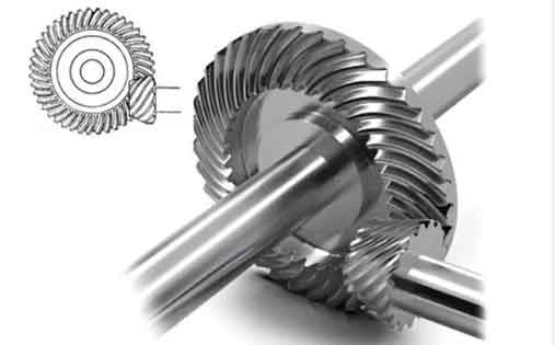
The pursuit of high-performance power transmission in intersecting-axis applications, such as automotive differentials, helicopter transmissions, and industrial reducers, has consistently driven advancements in gear technology. Among the various gear types, spiral bevel gears stand out due to their superior characteristics, including high contact ratio, smooth and quiet operation, and excellent load-carrying capacity. The performance and quality of these spiral bevel gears are paramount, directly influencing the technical and economic metrics of the host machinery. In recent years, the advent of digital closed-loop manufacturing, pioneered by companies like Gleason and Klingelnberg, has revolutionized the production of high-precision spiral bevel gears. This paradigm integrates computer-aided design, precision machining (milling/grinding), coordinate metrology, and error compensation software into a cohesive, iterative process aimed at ensuring the final manufactured tooth surface conforms precisely to its theoretical design, thereby guaranteeing pre-defined meshing performance.
Realizing this digital closed-loop manufacturing cycle hinges on solving several key technological challenges. The foremost among these is the establishment of a rigorous mathematical model for the theoretical tooth surface. This model must enable the calculation of spatial coordinates and normal vectors for a dense set of discrete points across the entire tooth flank, including both the working surface and the fillet region. These data are essential for subsequent steps: they provide the reference geometry for measuring deviations on a physical part and form the basis for the error correction algorithms that compute compensatory adjustments to the machine tool settings. This article, therefore, focuses on developing a comprehensive mathematical model for the full tooth surface of a spiral bevel gear, specifically for the pinion, based on the fundamental principles of its cutting process. The model explicitly incorporates modern machining corrections, such as cutter tilt and variable roll ratio, and establishes a robust method for surface discretization and point calculation, forming the indispensable foundation for the digital closed-loop manufacturing chain.
Fundamentals of Mathematical Modeling
The mathematical modeling of a generated gear tooth surface is intrinsically linked to its manufacturing simulation. For a spiral bevel gear pinion, the surface is enveloped by the family of surfaces traced by the cutting tool (cutter head) relative to the gear blank. We consider the case of a right-hand spiral pinion, noting that the methodology is analogous for a left-hand pinion or a generated gear member. The model accounts for the relative positioning and motion between the workpiece and the cutter on a hypoid gear generator, including essential correction motions.
Machine Coordinate System and Tool Geometry
The spatial relationship on the machine is defined within a coordinate system $\sigma_1 = { O_1; \mathbf{i}_1, \mathbf{j}_1, \mathbf{k}_1 }$, where $O_1$ is the machine center. The $\mathbf{i}_1-\mathbf{j}_1$ plane represents the machine plane, and $\mathbf{k}_1$ points into the cradle. The cutter head’s position is defined by the radial distance $S_1$ (machine center to cutter center) and the directional angle $q_1$ (cradle angle). The cutter axis orientation is defined by the basic cutter rotation angle $j$ and the cutter tilt angle $i$. The workpiece (gear blank) position is determined by several settings: the vertical offset $E_{m1}$, the sliding base setting $X_{B1}$, the machine root angle $\delta_{M1}$, and an axial positioning adjustment $X_1$.
The cutting edges of a duplex or single-point finishing cutter typically consist of two distinct sections: a straight-line segment with a specified pressure angle (or blade angle) $\alpha_{01}$, and a circular arc segment with a specified tip radius $r_e$. The straight segment generates the working tooth surface $\Sigma_1^{(a)}$, while the circular arc generates the root fillet transition surface $\Sigma_1^{(b)}$. As the cutter rotates about its own axis $\mathbf{c}$ with rotation angle $\theta_1$, these edges generate the tool surfaces: a conical surface $\Sigma_0^{(a)}$ and a toroidal surface $\Sigma_0^{(b)}$, respectively.
Development of the Comprehensive Tooth Surface Model
1. Equation of the Tool Cutting Surfaces
The geometry of the cutter is defined in its own coordinate system. Let $\mathbf{b}$ be the projection of the cutter axis $\mathbf{c}$ onto the machine plane. Its direction vector is:
$$\mathbf{b} = \sin(q_1 – j) \mathbf{i}_1 + \cos(q_1 – j) \mathbf{j}_1$$
The cutter axis vector $\mathbf{c}$ is then:
$$\mathbf{c} = \sin i \sin(q_1 – j) \mathbf{i}_1 + \sin i \cos(q_1 – j) \mathbf{j}_1 – \cos i \mathbf{k}_1$$
Conical Surface $\Sigma_0^{(a)}$: A point $M$ on the straight blade segment is defined by a distance parameter $s_1$ from the blade tip. The position vector of the blade tip $\mathbf{r’}^{(a)}_0$, the unit tangent vector along the blade $\mathbf{t’}^{(a)}_1$, and the unit normal vector $\mathbf{n’}^{(a)}_1$ in the initial blade section are derived from projections onto $\mathbf{b}$ and $\mathbf{k}_1$:
$$
\begin{aligned}
\mathbf{r’}^{(a)}_0 &= r_{01}[\cos i \sin(q_1-j) \mathbf{i}_1 + \cos i \cos(q_1-j) \mathbf{j}_1 + \sin i \mathbf{k}_1] \\
\mathbf{n’}^{(a)}_1 &= \cos(\alpha_{01}-i) \sin(q_1-j) \mathbf{i}_1 + \cos(\alpha_{01}-i) \cos(q_1-j) \mathbf{j}_1 – \sin(\alpha_{01}-i) \mathbf{k}_1 \\
\mathbf{t’}^{(a)}_1 &= \sin(\alpha_{01}-i) \sin(q_1-j) \mathbf{i}_1 + \sin(\alpha_{01}-i) \cos(q_1-j) \mathbf{j}_1 + \cos(\alpha_{01}-i) \mathbf{k}_1
\end{aligned}
$$
where $r_{01}$ is the cutter point radius. Rotating these vectors about the cutter axis $\mathbf{c}$ by the rotation angle $\theta_1$ gives the corresponding vectors for any axial section of the cutting surface:
$$
\begin{aligned}
\mathbf{r}^{(a)}_0 &= (\mathbf{c} \cdot \mathbf{r’}^{(a)}_0) \mathbf{c} + \cos\theta_1 (\mathbf{c} \times \mathbf{r’}^{(a)}_0) \times \mathbf{c} + \sin\theta_1 (\mathbf{c} \times \mathbf{r’}^{(a)}_0) \\
\mathbf{t}^{(a)}_1 &= (\mathbf{c} \cdot \mathbf{t’}^{(a)}_1) \mathbf{c} + \cos\theta_1 (\mathbf{c} \times \mathbf{t’}^{(a)}_1) \times \mathbf{c} + \sin\theta_1 (\mathbf{c} \times \mathbf{t’}^{(a)}_1) \\
\mathbf{n}^{(a)}_1 &= (\mathbf{c} \cdot \mathbf{n’}^{(a)}_1) \mathbf{c} + \cos\theta_1 (\mathbf{c} \times \mathbf{n’}^{(a)}_1) \times \mathbf{c} + \sin\theta_1 (\mathbf{c} \times \mathbf{n’}^{(a)}_1)
\end{aligned}
$$
The final equation for the conical cutting surface $\Sigma_0^{(a)}$ is:
$$\mathbf{r}^{(a)}_{c1} = S_1 \cos q_1 \mathbf{i}_1 – S_1 \sin q_1 \mathbf{j}_1 + \mathbf{r}^{(a)}_0 + s_1 \mathbf{t}^{(a)}_1$$
The parameter $s_1$ must be greater than or equal to $r_e \tan(\pi/4 – \alpha_{01}/2)$ to ensure the point is on the straight segment. For convex side cutting (using the inner blade), $\alpha_{01}$ is positive; for concave side cutting (outer blade), $\alpha_{01}$ is negative.
Toroidal Surface $\Sigma_0^{(b)}$: A point on the circular tip is defined by an angular parameter $\lambda_e$ measured from the end of the straight segment. The geometry involves the radius $r_w = r_{01} \pm r_e (1 – \sin \alpha_{01})/\cos \alpha_{01}$ and an auxiliary angle $\psi$. Following a similar derivation, the initial vectors for the circular segment are:
$$
\begin{aligned}
\mathbf{r’}^{(b)}_0 &= r_b[\cos(i+\psi) \sin(q_1-j) \mathbf{i}_1 + \cos(i+\psi) \cos(q_1-j) \mathbf{j}_1 + \sin(i+\psi) \mathbf{k}_1] \\
\mathbf{n’}^{(b)}_1 &= \sin(\lambda_e \mp i) \sin(q_1-j) \mathbf{i}_1 + \sin(\lambda_e \mp i) \cos(q_1-j) \mathbf{j}_1 \pm \cos(\lambda_e \mp i) \mathbf{k}_1 \\
\mathbf{t’}^{(b)}_1 &= \mp \cos(\lambda_e \mp i) \sin(q_1-j) \mathbf{i}_1 \mp \cos(\lambda_e \mp i) \cos(q_1-j) \mathbf{j}_1 + \sin(\lambda_e \mp i) \mathbf{k}_1
\end{aligned}
$$
where $r_b = \sqrt{(r_w \mp r_e \sin \lambda_e)^2 + r_e^2(1-\cos \lambda_e)^2}$. The upper sign corresponds to the inner blade (convex side generation) and the lower to the outer blade (concave side). Rotating by $\theta_1$ yields $\mathbf{r}^{(b)}_0$, $\mathbf{n}^{(b)}_1$, and $\mathbf{t}^{(b)}_1$. The toroidal cutting surface equation is:
$$\mathbf{r}^{(b)}_{c1} = S_1 \cos q_1 \mathbf{i}_1 – S_1 \sin q_1 \mathbf{j}_1 + \mathbf{r}^{(b)}_0$$
The parameter $\lambda_e$ ranges from $0$ to $\pi/2 – |\alpha_{01}|$.
2. Equation of the Generated Pinion Tooth Surface
The pinion tooth surface is the envelope of the family of cutting tool surfaces generated during the relative rolling motion between the imaginary generating gear (cradle) and the workpiece. The cradle rotates with angular velocity $\boldsymbol{\omega}_1 = -\mathbf{k}_1$. The workpiece rotation $\phi_1$ is related to the cradle rotation increment $\Delta q_1$ through a polynomial function that incorporates a variable roll ratio and high-order corrections (c, d, e, f):
$$\phi_1 = i_{01} (\Delta q_1 – c \Delta q_1^2 – d \Delta q_1^3 – e \Delta q_1^4 – f \Delta q_1^5)$$
where $i_{01}$ is the basic ratio of roll. The angular velocity and acceleration of the workpiece are:
$$\frac{d\phi_1}{dt} = i_{01}(1 – 2c\Delta q_1 – 3d\Delta q_1^2 – 4e\Delta q_1^3 – 5f\Delta q_1^4)$$
$$\frac{d^2\phi_1}{dt^2} = -i_{01}(2c + 6d\Delta q_1 + 12e\Delta q_1^2 + 20f\Delta q_1^3)$$
The relative velocity between the cutting surface and the workpiece at a potential contact point $M$ is crucial. For the conical surface $\Sigma_0^{(a)}$ acting as the generating surface, the relative velocity $\mathbf{v}_{12}^{(a)}$ is:
$$\mathbf{v}_{12}^{(a)} = \boldsymbol{\omega}_{12} \times \mathbf{r}^{(a)}_{c1} + \frac{d\phi_1}{dt} \mathbf{p}_1 \times \mathbf{m}_1$$
where $\boldsymbol{\omega}_{12} = -\mathbf{k}_1 + \frac{d\phi_1}{dt}\mathbf{p}_1$, $\mathbf{p}_1 = -\cos\delta_{M1}\mathbf{i}_1 + \sin\delta_{M1}\mathbf{k}_1$ is the pinion axis direction, and $\mathbf{m}_1 = X_1\mathbf{p}_1 – E_{m1}\mathbf{j}_1 + X_{B1}\mathbf{k}_1$ is the vector from the machine center to the pinion design crossing point.
The fundamental equation of meshing (contact condition) requires that the relative velocity is orthogonal to the common surface normal at the contact point: $\mathbf{v}_{12}^{(a)} \cdot \mathbf{n}^{(a)}_1 = 0$. Substituting the expressions leads to an equation that can be solved for the blade parameter $s_1$:
$$s_1 = – \frac{(\boldsymbol{\omega}_{12}, \mathbf{r}^{(a)}_0, \mathbf{n}^{(a)}_1) + \frac{d\phi_1}{dt} (\mathbf{p}_1, \mathbf{m}_1, \mathbf{n}^{(a)}_1)}{(\boldsymbol{\omega}_{12}, \mathbf{t}^{(a)}_1, \mathbf{n}^{(a)}_1)}$$
where $(\cdot,\cdot,\cdot)$ denotes the scalar triple product.
For the toroidal surface $\Sigma_0^{(b)}$, the meshing equation $\mathbf{v}_{12}^{(b)} \cdot \mathbf{n}^{(b)}_1 = 0$ yields a transcendental equation that can be solved for the parameter $\lambda_e$:
$$\lambda_e = \arctan(-C/S)$$
where $S$ and $C$ are lengthy expressions involving the machine settings, motion parameters, and the variables $\Delta q_1$ and $\theta_1$.
Substituting the solved parameters $s_1(\Delta q_1, \theta_1)$ or $\lambda_e(\Delta q_1, \theta_1)$ back into the respective cutting surface equations $\mathbf{r}^{(a)}_{c1}$ or $\mathbf{r}^{(b)}_{c1}$ gives the line of contact on the tool for a given cradle angle increment $\Delta q_1$. The family of all such contact lines, generated as $\Delta q_1$ varies, forms the pinion tooth surface. Finally, translating to the pinion coordinate system (origin at the crossing point $O’$), the equations for the working surface $\Sigma_1^{(a)}$ and the fillet surface $\Sigma_1^{(b)}$ are:
$$
\mathbf{r}^{(a)}_1 = \mathbf{r}^{(a)}_{c1} + \mathbf{m}_1, \quad \mathbf{r}^{(b)}_1 = \mathbf{r}^{(b)}_{c1} + \mathbf{m}_1
$$
The unit normal vectors on the pinion tooth surface at the point of generation are identical to those on the cutting tool at the same instant: $\mathbf{n}^{(a)}_1$ and $\mathbf{n}^{(b)}_1$, respectively.
Methodology for Tooth Surface Discretization and Point Calculation
For digital closed-loop manufacturing, the theoretical tooth surface defined by the above model must be discretized into a grid of points. Let $M$ be a point on the pinion tooth surface. Its location is conveniently described in a cylindrical coordinate system attached to the pinion: the radial distance $r_1$ from the pinion axis, and the axial coordinate $L_1$ along the pinion axis from the crossing point.
$$
r_1 = |\mathbf{r}_1 \times \mathbf{p}_1|, \quad L_1 = \mathbf{r}_1 \cdot \mathbf{p}_1
$$
where $\mathbf{r}_1$ is either $\mathbf{r}^{(a)}_1$ or $\mathbf{r}^{(b)}_1$. For a given pair of machine motion parameters $(\Delta q_1, \theta_1)$, one can compute the corresponding $(r_1, L_1)$. Conversely, to find the coordinates and normal vector of a specific point on the designed surface defined by a given $(r_1, L_1)$, one must solve the inverse problem: find the parameters $(\Delta q_1, \theta_1)$ that satisfy the surface equations and the coordinate conditions. This is typically achieved using a numerical root-finding method like the Newton-Raphson iteration for two variables.
The practical procedure is as follows:
- Grid Definition: A grid is overlaid on the tooth surface in a domain defined by the tooth length (from heel to toe) and tooth depth (from tip to root/fillet). This grid can be defined in terms of $(r_1, L_1)$ coordinates.
- Parameter Solution: For each grid node $(r_{1,ij}, L_{1,ij})$, the Newton-Raphson method is applied to the system of equations $F(\Delta q_1, \theta_1) = r_1(\Delta q_1, \theta_1) – r_{1,ij} = 0$ and $G(\Delta q_1, \theta_1) = L_1(\Delta q_1, \theta_1) – L_{1,ij} = 0$ to find the corresponding $(\Delta q_{1,ij}, \theta_{1,ij})$.
- Coordinate & Normal Calculation: The solved parameters are substituted into the surface equations $\mathbf{r}_1(\Delta q_{1,ij}, \theta_{1,ij})$ and $\mathbf{n}_1(\Delta q_{1,ij}, \theta_{1,ij})$ to obtain the 3D Cartesian coordinates $(X, Y, Z)$ and the unit normal vector components $(N_x, N_y, N_z)$ for that discrete point.
This process yields a complete digital twin of the tooth surface, essential for measurement path planning and error evaluation in closed-loop manufacturing of spiral bevel gears.
Application Example and Model Verification
To validate the developed mathematical model and the discretization algorithm, we consider a spiral bevel gear pair from a reducer. The basic gear geometry and the specific machine settings for cutting the pinion are listed below.
| Parameter | Value |
|---|---|
| Gear Ratio | 48 / 55 |
| Transverse Module, $m_{et}$ (mm) | 3 |
| Normal Pressure Angle, $\alpha_n$ (°) | 20 |
| Mean Spiral Angle, $\beta_m$ (°) | 30 |
| Face Width, $b$ (mm) | 22 |
| Parameter | Concave Side | Convex Side |
|---|---|---|
| Radial Setting, $S_1$ (mm) | 98.3171 | 93.8550 |
| Cradle Angle, $q_1$ (°) | 61.72 | 55.89 |
| Cutter Tilt Angle, $i$ (°) | 0.0 | 0.0 |
| Basic Cutter Rotation, $j$ (°) | 30.10 | 26.53 |
| Machine Root Angle, $\delta_{M1}$ (°) | 39.15 | 39.15 |
| Sliding Base, $X_{B1}$ (mm) | -0.1943 | 0.2990 |
| Axial Position, $X_1$ (mm) | 1.1470 | 0.3655 |
| Vertical Offset, $E_{m1}$ (mm) | 0.0 | 0.0 |
| Ratio of Roll, $R_a$ | 1.539737 | 1.517470 |
| Cutter Point Radius, $r_{01}$ (mm) | 97.94 | 112.65 |
| Blade Angle, $\alpha_{01}$ (°) | 18.75 | 21.25 |
Using the described methodology, the pinion tooth surfaces were discretized into a 9×5 grid (9 points along the length, 5 points along the profile). The computed Cartesian coordinates and unit normal vectors for points on both the convex and concave flanks are presented below. The consistency and realism of these values serve as a primary verification of the model’s correctness.
| Grid (J,I) | X (mm) | Y (mm) | Z (mm) | Nx | Ny | Nz |
|---|---|---|---|---|---|---|
| (1,1) | 68.6130 | -4.6493 | -82.3985 | 0.6091 | 0.7667 | -0.2028 |
| (1,2) | 69.4204 | -5.1223 | -81.6665 | 0.6323 | 0.7522 | -0.1855 |
| … | … | … | … | … | … | … |
| (9,5) | 59.9545 | 3.9132 | -66.6210 | 0.5024 | 0.8618 | -0.0692 |
| Grid (J,I) | X (mm) | Y (mm) | Z (mm) | Nx | Ny | Nz |
|---|---|---|---|---|---|---|
| (1,1) | 68.4594 | -6.3272 | -82.4152 | -0.1967 | -0.7970 | 0.5711 |
| (1,2) | 69.3367 | -5.9879 | -81.6791 | -0.1670 | -0.7887 | 0.5916 |
| … | … | … | … | … | … | … |
| (9,5) | 59.8442 | 5.3428 | -66.6212 | 0.0778 | -0.8143 | 0.5752 |
The complete set of computed discrete points can be exported to CAD/CAM software to reconstruct a 3D solid model of the pinion, providing a visual and geometric confirmation of the model’s validity. This model serves as the absolute digital reference for all subsequent steps in the digital closed-loop manufacturing process for these spiral bevel gears.
Conclusion
This work has successfully established a comprehensive mathematical framework for modeling the full tooth surface of spiral bevel gears, specifically tailored to the requirements of digital closed-loop manufacturing. The key accomplishments are summarized as follows:
- Integrated Mathematical Model: A model was derived from first principles of gear generation, incorporating the detailed geometry of the cutting tool (straight and circular edges) and the precise kinematic relationship between the workpiece and the cutter on a modern hypoid generator. Critical process corrections, namely cutter tilt ($i$) and higher-order roll ratio modifications (via coefficients $c, d, e, f$), were explicitly included in the formulation, enhancing the model’s accuracy and relevance to advanced finishing processes.
- Complete Surface Description: The model provides explicit equations for both the working tooth surface $\Sigma_1^{(a)}$ and the root fillet transition surface $\Sigma_1^{(b)}$. This full-tooth modeling is crucial for accurate stress analysis and for ensuring proper clearance in the final gear assembly.
- Discretization and Inverse Calculation Algorithm: A robust methodology was established for discretizing the complex, parametrically defined tooth surface. The method involves defining a surface grid in convenient pinion coordinates ($r_1, L_1$) and employing a numerical root-finding technique to solve for the corresponding machine motion parameters ($\Delta q_1, \theta_1$). This allows for the direct calculation of the 3D coordinates $(X, Y, Z)$ and the unit normal vector $(N_x, N_y, N_z)$ for any specified point on the designed tooth surface.
- Foundation for Digital Closed-Loop Manufacturing: The generated set of discrete points with their associated normals constitutes the essential digital twin of the gear. This dataset is the fundamental input for generating inspection paths on a gear measuring center or CMM, and for computing the deviation between the theoretical and manufactured surfaces. These deviations are then fed into error compensation software to calculate corrective adjustments to the machine settings, closing the digital loop.
Therefore, the developed model and algorithms form the critical first pillar in the digital closed-loop manufacturing system for high-precision spiral bevel gears. By providing a rigorous, computable definition of the target geometry, it enables the precise control and iterative refinement necessary to achieve optimal contact patterns, low noise, and high durability in final gear products, meeting the ever-increasing demands of modern powertrain systems.