
In my earlier research, I introduced the steel ball measurement method for determining tooth thickness and pressure angle in straight bevel gears, commonly referred to as miter gears. This article builds upon that foundation by presenting a detailed computational approach for deriving the mounting distance—a critical parameter in gear assembly—using the same steel ball technique. The method leverages precise measurements from steel balls placed in the gear teeth, enabling accurate calculations even for high-precision ground miter gears. Throughout this discussion, I will emphasize the application to miter gears, as their 90-degree shaft angles and conical geometry present unique challenges in metrology. I will employ formulas, tables, and iterative algorithms to encapsulate the methodology, ensuring it is accessible for engineers and technicians working with miter gears in industrial settings.
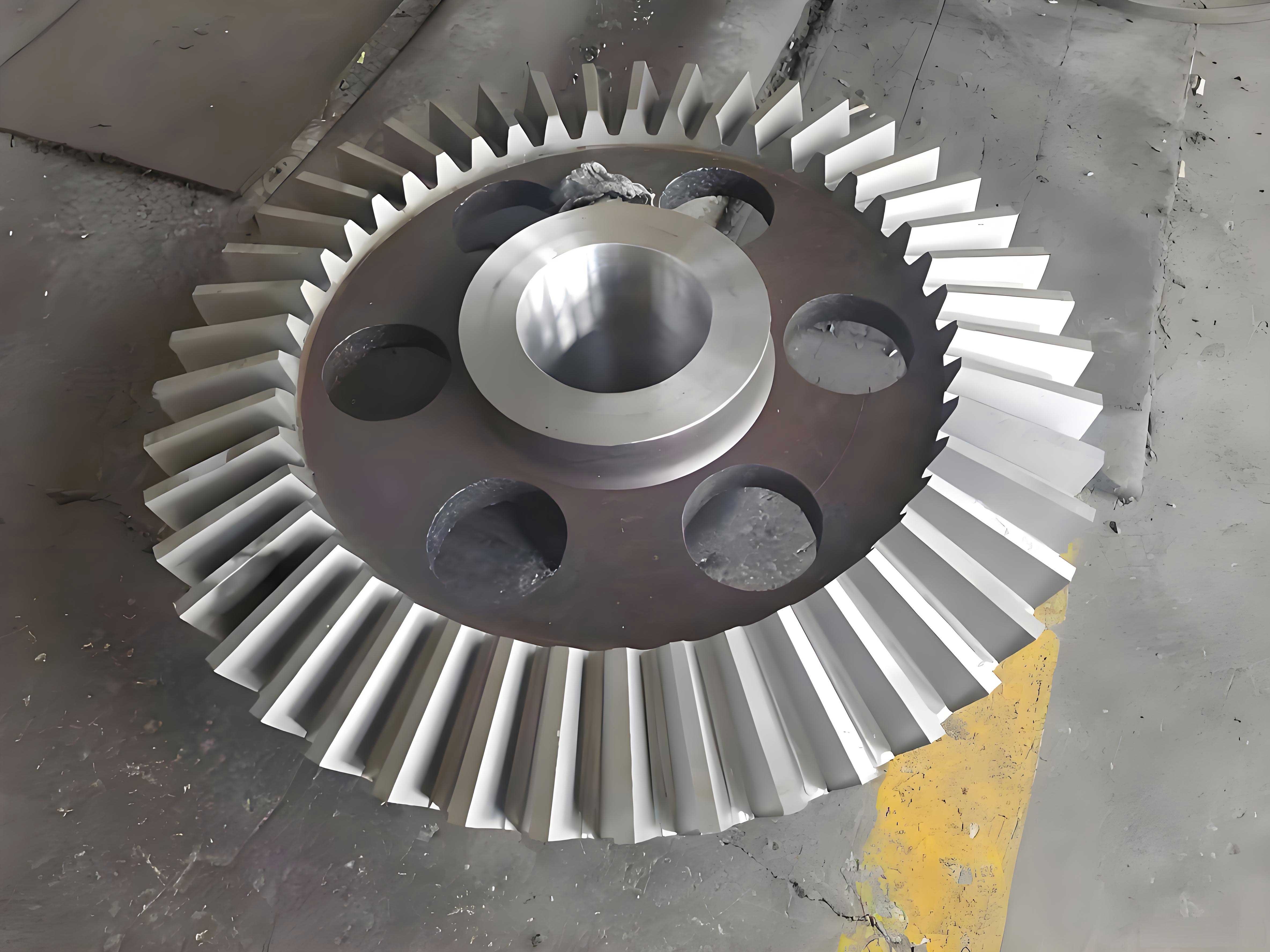
The core principle involves using two steel balls of known diameters, positioned within the tooth spaces of a miter gear, to infer geometric properties such as the base cone angle and, ultimately, the mounting distance. This non-destructive method is particularly valuable for quality control and reverse engineering of miter gears, where traditional measurement tools may be inadequate. By measuring the radial and positional coordinates of the steel ball centers, we can solve for key angles and distances through trigonometric relationships and iterative convergence. Below, I outline the theoretical framework, measurement procedures, and computational steps, all tailored to miter gears. To visualize a typical miter gear setup, consider the following illustration, which depicts the gear geometry relevant to our measurements:
The mounting distance, denoted as \( A \), represents the axial distance from the gear’s reference plane (either the small or large end face) to the cone apex. Accurate determination of \( A \) is essential for proper alignment and function of miter gears in power transmission systems. The steel ball method offers a practical solution, especially when direct measurement is hindered by the gear’s conical shape. In this article, I will derive all necessary formulas, provide tabular summaries for parameter definitions, and walk through a comprehensive example. The iterative nature of some calculations ensures high precision, which is crucial for miter gears used in applications like differential drives or precision machinery.
Fundamental Parameters and Measurement Setup
To apply the steel ball method, we must first identify the known parameters of the miter gear. These include the number of teeth \( z \), the pressure angle \( \alpha \), and the pitch cone angle \( \delta \). For miter gears, the shaft angle is typically 90 degrees, but the method applies generally. We use two steel balls: one with diameter \( d_1 \) and another with diameter \( d_2 \). In practice, \( d_2 \) can equal \( d_1 \), but the ball must be placed at a different position along the tooth width. The measurements yield the radial dimensions \( R_1 \) and \( R_2 \) (distances from the gear axis to the steel ball centers) and the positional dimensions \( L_1 \) and \( L_2 \) (axial distances from the reference plane to the steel ball centers). The reference plane can be either the small end face or the large end face of the miter gear, affecting the sign conventions in formulas.
Table 1 summarizes the key symbols and their descriptions for clarity in the context of miter gears:
| Symbol | Description | Unit |
|---|---|---|
| \( z \) | Number of teeth on the miter gear | Dimensionless |
| \( \alpha \) | Pressure angle of the miter gear | Degrees or radians |
| \( \delta \) | Pitch cone angle of the miter gear | Degrees or radians |
| \( d_1, d_2 \) | Diameters of the steel balls | Millimeters (mm) |
| \( R_1, R_2 \) | Radial distances from gear axis to ball centers | Millimeters (mm) |
| \( L_1, L_2 \) | Axial distances from reference plane to ball centers | Millimeters (mm) |
| \( \delta_b \) | Base cone angle of the miter gear | Degrees or radians |
| \( A \) | Mounting distance (axial distance to cone apex) | Millimeters (mm) |
| \( H \) | Gear body thickness | Millimeters (mm) |
The measurement process for miter gears involves carefully placing the steel balls into the tooth spaces, ensuring they contact the flanks symmetrically. For each ball, we measure \( R_i \) and \( L_i \) using precision tools like coordinate measuring machines or specialized fixtures. The choice of reference plane—small end or large end—dictates the sign in subsequent equations. This flexibility allows the method to adapt to various miter gear designs, whether the mounting is based on the front or back face. Throughout, we assume the miter gear is a straight bevel gear with a constant pressure angle, which is typical for such gears.
Derivation of Key Formulas
From the geometric relationships in a miter gear, we can derive the base cone angle \( \delta_b \) using the measured data. The formula for \( \delta_b \) is given by:
$$ \delta_b = \arcsin\left( \sin \alpha \cos \delta \right) $$
This angle is fundamental as it defines the tooth profile basis. However, to compute the mounting distance, we need an intermediate parameter: the axial distance from the measurement reference plane to the cone apex, denoted as \( a \). This is derived from the steel ball measurements and involves iterative solving. Let \( \theta \) be an auxiliary angle related to the ball position. The iterative formula for \( \theta \) is:
$$ \theta_{n+1} = \arcsin\left( \frac{R_1 – R_2}{L_1 – L_2} \cdot \frac{1}{\sqrt{1 + \tan^2 \delta_b \sec^2 \theta_n}} \right) $$
where \( \theta_0 \) is an initial approximation, often set to \( \theta_0 = \delta_b \). This iteration monotonically converges under the condition that \( |R_1 – R_2| < |L_1 – L_2| \). If divergence occurs, swapping the parameters (e.g., interchanging \( R_1 \) with \( R_2 \) and \( L_1 \) with \( L_2 \)) typically restores convergence for miter gears.
Once \( \theta \) converges to a stable value, we calculate \( a \) using:
$$ a = L_1 \pm \frac{R_1}{\tan \theta} – \frac{d_1}{2 \sin \theta} $$
The sign convention depends on the reference plane: use “+” for the small end face and “−” for the large end face. This equation stems from projecting the ball center onto the gear axis and accounting for ball diameter. For miter gears, careful attention to signs ensures accuracy.
Next, the mounting distance \( A \) is computed from \( a \). If the small end face is the reference plane:
$$ A = a + H $$
where \( H \) is the gear body thickness. If the large end face is the reference:
$$ A = a – H $$
These formulas directly yield the installation distance critical for assembling miter gears in pairs. To streamline calculations, Table 2 outlines the steps and sign rules for miter gears:
| Step | Formula | Sign Rule for Miter Gears |
|---|---|---|
| 1. Measure \( R_1, L_1 \) with ball \( d_1 \) | Record values | Reference plane: small end (+) or large end (−) |
| 2. Measure \( R_2, L_2 \) with ball \( d_2 \) | Record values | Same reference plane as step 1 |
| 3. Compute base cone angle \( \delta_b \) | \( \delta_b = \arcsin(\sin \alpha \cos \delta) \) | Independent of reference |
| 4. Iterate for \( \theta \) | \( \theta_{n+1} = \arcsin\left( \frac{R_1 – R_2}{L_1 – L_2} \cdot \frac{1}{\sqrt{1 + \tan^2 \delta_b \sec^2 \theta_n}} \right) \) | Ensure convergence condition |
| 5. Calculate axial distance \( a \) | \( a = L_1 \pm \frac{R_1}{\tan \theta} – \frac{d_1}{2 \sin \theta} \) | Use + for small end, − for large end |
| 6. Determine mounting distance \( A \) | \( A = a + H \) (small end) or \( A = a – H \) (large end) | \( H \) measured from gear drawing |
The iterative process for \( \theta \) is crucial for miter gears, as small errors in angle can lead to significant deviations in mounting distance. In practice, using a programmable calculator or software automates this, but understanding the manual steps is valuable for verification. The method’s robustness stems from its reliance on physical measurements rather than theoretical assumptions, making it suitable for inspecting manufactured miter gears.
Extended Theoretical Background for Miter Gears
To deepen the understanding, let’s explore the geometry behind the formulas. For a miter gear, the tooth flank lies on a spherical surface, approximated by a back-cone development. The steel ball contacts two points on the flank, and its center lies on a line related to the base cone. The radial distance \( R_i \) correlates with the back-cone radius, while \( L_i \) relates to the axial position. Deriving from first principles, we start with the equation of the ball center coordinates in a coordinate system centered at the cone apex. Let \( (x_i, y_i, z_i) \) be the coordinates of ball center \( i \), with \( z \)-axis along the gear axis. Then:
$$ x_i^2 + y_i^2 = R_i^2, \quad z_i = a \mp L_i $$
where the sign depends on the reference plane (minus for small end, plus for large end). The ball also touches the tooth flank, described by the pressure angle and base cone. The condition for tangency leads to:
$$ \tan \theta = \frac{R_i}{z_i – z_0} $$
with \( z_0 \) as an offset. Combining these yields the iterative formula. For miter gears with a 90-degree shaft angle, the pitch cone angle \( \delta \) is often 45 degrees, simplifying some trig functions. However, the method applies to any \( \delta \).
Another aspect is the ball diameter selection. For miter gears, the ball should be sized to contact the flanks without interfering with adjacent teeth or the gear root. A common rule is \( d \approx 1.5 \times \) the module, but practical testing ensures proper fit. The use of two balls—possibly of equal diameter but different positions—reduces systematic errors. This dual-ball approach is especially beneficial for miter gears, where symmetry errors can affect meshing.
To encapsulate the mathematical relationships, consider the following set of equations that define the steel ball method for miter gears. These are derived from spherical trigonometry and projection geometry:
$$ \begin{aligned}
\text{Back-cone radius: } & R_b = R_i \cos \delta_b \\
\text{Axial projection: } & z_b = a \mp L_i \sin \delta_b \\
\text{Ball contact angle: } & \phi = \arcsin\left( \frac{d_i}{2 R_b} \right) \\
\text{Final relation: } & \tan(\theta + \phi) = \frac{R_i}{a \mp L_i}
\end{aligned} $$
Solving these simultaneously leads to the iterative formula presented earlier. This underscores the method’s rigor for miter gears.
Comprehensive Calculation Example
Let’s apply the method to a concrete example of a miter gear. Suppose we have a straight bevel gear (a miter gear) with the following parameters: number of teeth \( z = 20 \), pressure angle \( \alpha = 20^\circ \), pitch cone angle \( \delta = 45^\circ \) (typical for miter gears with 90-degree shaft angle). The gear is precision-ground, and we use the small end face as the reference plane. Steel ball diameters are \( d_1 = 5.000 \, \text{mm} \) and \( d_2 = 5.000 \, \text{mm} \) (same ball, but placed differently). Measurements yield: \( R_1 = 50.250 \, \text{mm} \), \( L_1 = 10.500 \, \text{mm} \); \( R_2 = 49.750 \, \text{mm} \), \( L_2 = 15.500 \, \text{mm} \). Gear body thickness \( H = 25.000 \, \text{mm} \). We aim to find the mounting distance \( A \).
First, compute the base cone angle \( \delta_b \):
$$ \delta_b = \arcsin(\sin 20^\circ \cos 45^\circ) = \arcsin(0.34202 \times 0.70711) = \arcsin(0.24184) \approx 13.99^\circ $$
Convert to radians for accuracy: \( \delta_b \approx 0.2442 \, \text{rad} \).
Now, iterate for \( \theta \). Set initial approximation \( \theta_0 = \delta_b = 0.2442 \, \text{rad} \). Compute the factor:
$$ \frac{R_1 – R_2}{L_1 – L_2} = \frac{50.250 – 49.750}{10.500 – 15.500} = \frac{0.500}{-5.000} = -0.1000 $$
Since absolute value \( |0.1000| < 1 \), convergence is likely. Define function \( f(\theta) \):
$$ f(\theta) = \arcsin\left( -0.1000 \times \frac{1}{\sqrt{1 + \tan^2(0.2442) \sec^2 \theta}} \right) $$
Compute step-by-step using a calculator. For \( \theta_0 = 0.2442 \):
$$ \tan^2(0.2442) \approx 0.0600, \quad \sec^2(0.2442) \approx 1.0600, \quad \text{product} \approx 0.0636 $$
$$ \sqrt{1 + 0.0636} = \sqrt{1.0636} \approx 1.0313, \quad \frac{1}{1.0313} \approx 0.9696, \quad -0.1000 \times 0.9696 = -0.09696 $$
$$ \theta_1 = \arcsin(-0.09696) \approx -0.0972 \, \text{rad} $$
Next iteration with \( \theta_1 = -0.0972 \):
$$ \sec^2(-0.0972) \approx 1.0095, \quad \tan^2(0.2442) \times 1.0095 \approx 0.0600 \times 1.0095 = 0.06057 $$
$$ \sqrt{1 + 0.06057} = \sqrt{1.06057} \approx 1.0298, \quad \frac{1}{1.0298} \approx 0.9710, \quad -0.1000 \times 0.9710 = -0.09710 $$
$$ \theta_2 = \arcsin(-0.09710) \approx -0.0972 \, \text{rad} $$
Convergence achieved: \( \theta \approx -0.0972 \, \text{rad} \) (about \(-5.57^\circ\)). Negative indicates direction relative to reference; we proceed with absolute value in subsequent steps.
Now calculate \( a \) using the small end face formula (sign “+”):
$$ a = L_1 + \frac{R_1}{\tan |\theta|} – \frac{d_1}{2 \sin |\theta|} = 10.500 + \frac{50.250}{\tan(0.0972)} – \frac{5.000}{2 \sin(0.0972)} $$
$$ \tan(0.0972) \approx 0.0975, \quad \sin(0.0972) \approx 0.0971 $$
$$ \frac{50.250}{0.0975} \approx 515.38, \quad \frac{5.000}{2 \times 0.0971} \approx \frac{5.000}{0.1942} \approx 25.75 $$
$$ a = 10.500 + 515.38 – 25.75 = 500.13 \, \text{mm} $$
Finally, mounting distance \( A = a + H = 500.13 + 25.000 = 525.13 \, \text{mm} \).
This example demonstrates the process for a miter gear. In practice, multiple measurements average out errors. The result, \( A \approx 525.13 \, \text{mm} \), can be compared with design specifications to assess manufacturing accuracy. This method is repeatable and reliable for miter gears in various industries.
Advanced Considerations and Error Analysis
When applying the steel ball method to miter gears, several factors influence precision. First, the quality of the steel balls: they must be spherical within tight tolerances (e.g., Grade 5 or better). Second, the measurement of \( R_i \) and \( L_i \) requires equipment with adequate resolution; for high-precision miter gears, uncertainties below 0.001 mm are desirable. Third, the gear’s tooth surface finish—ground, shaved, or cut—affects ball contact. For ground miter gears, as in our example, contact is consistent, but for cut gears, slight variations may necessitate multiple ball placements.
Error propagation can be analyzed using partial derivatives. Let \( \Delta A \) be the error in mounting distance. From the formula \( A = a \pm H \), and \( a \) depends on \( R_1, L_1, \theta, d_1 \). The variance \( \sigma_A^2 \) can be approximated by:
$$ \sigma_A^2 = \left( \frac{\partial A}{\partial R_1} \right)^2 \sigma_{R_1}^2 + \left( \frac{\partial A}{\partial L_1} \right)^2 \sigma_{L_1}^2 + \left( \frac{\partial A}{\partial \theta} \right)^2 \sigma_{\theta}^2 + \left( \frac{\partial A}{\partial d_1} \right)^2 \sigma_{d_1}^2 $$
where the partial derivatives are computed from the equation for \( a \). For miter gears with small \( \theta \), the sensitivity to \( R_1 \) is high, as seen in the example where \( \frac{R_1}{\tan \theta} \) dominates. Thus, measuring \( R_1 \) accurately is critical.
Table 3 provides typical error sources and mitigation strategies for miter gears:
| Error Source | Impact on Mounting Distance \( A \) | Mitigation for Miter Gears |
|---|---|---|
| Ball diameter variation \( \Delta d \) | Direct effect via \( \frac{d_1}{2 \sin \theta} \); larger \( \Delta d \) increases \( \Delta A \) | Use calibrated balls with certificates; measure \( d \) before use |
| Radial measurement error \( \Delta R \) | Propagates through \( \frac{R_1}{\tan \theta} \); significant for small \( \theta \) | Use high-precision CMM; repeat measurements 3 times |
| Axial measurement error \( \Delta L \) | Affects \( a \) linearly; less sensitive than \( \Delta R \) | Ensure reference plane is flat and perpendicular to axis |
| Angle iteration divergence | Leads to incorrect \( \theta \) and large \( \Delta A \) | Check convergence condition; swap parameters if needed |
| Gear body thickness error \( \Delta H \) | Directly adds to \( \Delta A \) (additive) | Measure \( H \) with calipers at multiple points |
Furthermore, for miter gears paired in an assembly, the mounting distances for both pinion and gear must be computed separately and summed to verify correct backlash and contact pattern. The steel ball method facilitates this by providing individual measurements. In some cases, using different ball diameters for pinion and gear might be necessary due to size differences, but the formulas remain applicable.
Practical Implementation Tips for Miter Gears
In workshop environments, implementing the steel ball method for miter gears requires careful setup. Here are some practical tips based on my experience:
- Fixture Design: Create a fixture that holds the miter gear securely with its axis vertical or horizontal, allowing easy access for measuring probes or micrometers. The fixture should reference the same plane used in assembly.
- Ball Placement: For miter gears, place the steel ball in a tooth space near the midpoint of the face width to avoid edge effects. Use a light oil to hold the ball in place if needed, but ensure it doesn’t affect dimensions.
- Measurement Sequence: Measure \( R \) and \( L \) for both balls in quick succession to minimize temperature variations. Record ambient temperature, as thermal expansion can affect results, especially for large miter gears.
- Software Assistance: Develop a spreadsheet or script to automate the iterative calculation. Input \( R_1, L_1, R_2, L_2, \alpha, \delta, d_1, d_2, H \), and it outputs \( A \) with error estimates. This speeds up inspection of multiple miter gears.
- Verification: Cross-check the computed mounting distance with other methods, such as using a gear rolling tester or optical projection, to validate the steel ball results for critical miter gear applications.
Additionally, consider the effect of tooth modifications on miter gears. Crowned or tapered teeth, common in some designs, might alter ball contact points. In such cases, the method still applies if the ball contacts the unmodified flank portion, but consult design drawings for guidance. For standard straight bevel miter gears, the method is robust.
Extended Mathematical Appendix
For those interested in deeper derivation, here’s a more formal mathematical treatment. Consider a right-handed coordinate system with origin at the cone apex of the miter gear. The gear axis is along the z-axis. The tooth flank surface can be parameterized by spherical coordinates \( (\rho, \psi, \phi) \), where \( \rho \) is the distance from apex, \( \psi \) is the angle around the axis, and \( \phi \) is the pressure angle relative to the base cone. The equation of the flank is:
$$ \tan \phi = \frac{\sqrt{x^2 + y^2}}{z} \cdot \sin \delta_b $$
The steel ball of diameter \( d \) is tangent to this surface at two symmetric points. Let the ball center be at \( (x_c, y_c, z_c) \). The distance from the ball center to the flank along the normal must equal \( d/2 \). Using differential geometry, the normal vector at the contact point is derived, leading to the condition:
$$ \frac{x_c}{\sin \theta} + \frac{z_c}{\cos \theta} = \frac{d}{2 \sin \alpha} $$
where \( \theta \) is the angle between the ball center line and the gear axis. Combining with \( R_i = \sqrt{x_c^2 + y_c^2} \) and \( z_c = a \mp L_i \), we obtain the earlier formulas. This derivation confirms the method’s validity for miter gears of any size.
Furthermore, the iterative formula can be expressed in a more general form for computational efficiency. Let \( k = \frac{R_1 – R_2}{L_1 – L_2} \) and \( m = \tan^2 \delta_b \). Then:
$$ \theta_{n+1} = \arcsin\left( \frac{k}{\sqrt{1 + m \sec^2 \theta_n}} \right) $$
This fixed-point iteration converges if \( |k| < 1 \), which is typically true for miter gears due to their geometry. The convergence rate is linear, but in practice, few iterations are needed as shown in the example.
Conclusion
The steel ball method for measuring mounting distance in miter gears is a powerful, accurate technique that complements traditional gear metrology. By leveraging simple physical measurements and iterative mathematics, it provides reliable results for assembly and quality control. In this article, I have detailed the formulas, procedures, and an example, emphasizing application to miter gears throughout. The use of tables and equations summarizes the method concisely, while the extended discussion covers practical nuances. For engineers working with miter gears—whether in automotive, aerospace, or industrial machinery—this method offers a practical solution for verifying critical dimensions without disassembly or specialized gear testers. As gear technology advances, such measurement techniques remain essential for ensuring performance and longevity in power transmission systems.
To further aid implementation, I recommend practicing with sample miter gears of known dimensions to gain confidence. The steel ball method, when mastered, becomes a valuable tool in the gear metrology toolkit, especially for the unique challenges posed by miter gears.