
My research is directed toward complex modified face gears, which are increasingly used in high-end transmission systems because they can transfer motion and torque between intersecting axes with high power density, large contact ratio, stable transmission ratio, and relatively low sensitivity to installation errors. In my work, I treat the face gear pair as a coupled geometric and mechanical system. I propose a tooth surface modification method that introduces explicit modification curve parameters, I build numerical models of the modified face gear pair, I analyze meshing characteristics through tooth contact analysis and loaded tooth contact analysis, and I optimize the modification parameters using a hybrid prediction and multi-objective optimization framework. The central aim is to improve contact position, reduce transmission error, and lower contact stress in complex modified face gears.
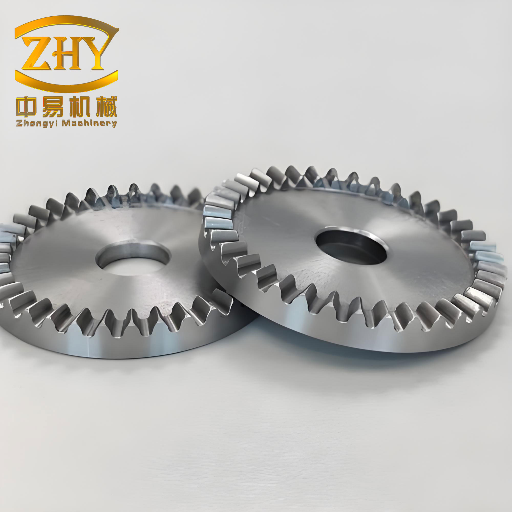
Face gears differ from conventional cylindrical gears because their teeth are distributed on an end face and their tooth surfaces are generated by a shaper cutter or a virtual generating gear. This geometry makes face gears highly attractive for aerospace and helicopter main reducers, but it also makes modification and modeling more difficult. The tooth surface of a face gear is not a simple involute surface. It changes continuously along the tooth width and tooth height. Therefore, a modification method developed for cylindrical gears cannot be transferred directly to face gears without considering the gradual variation of the face gear tooth surface. I address this problem by introducing modification curve parameters that separately control the inner and outer parts of the face gear tooth surface.
I begin with the standard generation principle of face gears. The shaper cutter is treated as a special spur gear with a standard involute profile. The tooth surface of the shaper cutter can be written as
$$ \mathbf{r}_s(u_s,\theta_s) = \begin{bmatrix} r_b[\sin(\theta_{os}+\theta_s) – \theta_s\cos(\theta_{os}+\theta_s)] \\ r_b[\cos(\theta_{os}+\theta_s) + \theta_s\sin(\theta_{os}+\theta_s)] \\ u_s \\ 1 \end{bmatrix} $$
where \(r_b\) is the base circle radius, \(\theta_s\) is the involute roll angle, \(\theta_{os}\) is the involute angle at the addendum, and \(u_s\) is the tooth width parameter of the shaper cutter. The plus and minus signs correspond to the right and left flanks of the shaper cutter, respectively. For face gears, the working tooth surface is generated as the envelope of the shaper cutter tooth surface during a relative motion. The coordinate transformation from the shaper cutter coordinate system to the face gear coordinate system is expressed by a matrix \(\mathbf{M}_{2s}(\phi_s)\). The family of shaper cutter surfaces in the face gear coordinate system is
$$ \mathbf{r}_2(u_s,\theta_s,\phi_s) = \mathbf{M}_{2s}(\phi_s)\mathbf{r}_s(u_s,\theta_s) $$
The meshing equation that relates the motion parameter and the geometric parameters is
$$ f(u_s,\theta_s,\phi_s) = \mathbf{n}_s \cdot \mathbf{v}_s^{(2s)} = 0 $$
For a face gear generated by a spur shaper cutter, this meshing equation can be simplified to
$$ f(u_s,\theta_s,\phi_s) = r_b – u_s m_{2s}\cos(\theta_s + \theta_{os} + \phi_s) = 0 $$
where \(m_{2s}\) is the gear ratio between the shaper cutter and the face gear. Eliminating \(u_s\) from the family of surfaces and the meshing equation gives the working tooth surface of the face gear:
$$ \mathbf{r}_2(\theta_s,\phi_s) = \begin{bmatrix} x_2 \\ y_2 \\ z_2 \\ 1 \end{bmatrix} = \begin{bmatrix} \frac{r_b}{\cos\phi_s}[\sin\psi – \psi\cos\psi] \\ -\frac{r_b}{\cos\phi_s}[\cos\psi + \psi\sin\psi] \\ -r_b[\cos\psi + \psi\sin\psi] \\ 1 \end{bmatrix} $$
where \(\psi = \theta_{os} + \theta_s + \phi_s\). The transition surface of the face gear is generated by the addendum edge of the shaper cutter and does not participate in meshing. It connects the working tooth surface with the root region and is important for the mechanical integrity of face gears. The transition curve can be obtained by substituting the addendum involute parameter into the meshing equation. The complete face gear tooth surface therefore consists of a working surface, a transition surface, and a transition curve.
The basic geometric parameters I use for the face gear pair are summarized in Table 1. These parameters define the shaper cutter, the cylindrical pinion, and the face gear. I use them consistently in the generation, modification, contact analysis, and optimization procedures.
| Parameter | Symbol | Value |
|---|---|---|
| Number of teeth of cylindrical pinion | \(N_1\) | 21 |
| Number of teeth of shaper cutter | \(N_s\) | 23 |
| Number of teeth of face gear | \(N_2\) | 48 |
| Pressure angle | \(\alpha\) | \(25^\circ\) |
| Shaft angle | \(\gamma\) | \(90^\circ\) |
| Module | \(m\) | 3.9 mm |
| Inner radius of face gear | \(L_1\) | 180 mm |
| Outer radius of face gear | \(L_2\) | 200 mm |
After establishing the standard face gear tooth surface, I introduce the modification method. For cylindrical gears, crowning modification is widely used. A common parabolic crowning curve is
$$ \Delta c = \alpha_0 u^2 $$
where \(\alpha_0\) is the crowning coefficient and \(u\) is the position parameter along the tooth width. For face gears, however, the tooth surface changes continuously from the inner end to the outer end. A single symmetric crowning curve is not sufficient. I therefore define a modification method with two curve parameters, \(K_1\) and \(K_2\), that act on the outer and inner parts of the face gear tooth surface, respectively. The modification amount at a point on the face gear tooth surface is
$$ \Delta = \begin{cases} K_1 \alpha_0 u_m^2, & 0.5 \leq K_1 \leq 1.0 \\ K_2 \alpha_0 u_m^2, & 1.0 \leq K_2 \leq 1.5 \end{cases} $$
where \(u_m\) is the position parameter along the tooth width direction. The outer part uses \(K_1\) in the range \(0.5\) to \(1.0\), which avoids unnecessary material removal and reduces the risk of edge contact. The inner part uses \(K_2\) in the range \(1.0\) to \(1.5\), which distributes contact stress more effectively and reduces the risk of fatigue or wear at the inner end. This strategy ensures that the modification amount is smaller at the outer end and larger at the inner end, producing a gradual transition over the face gear tooth surface.
For the cylindrical pinion, I apply both profile modification and lead modification. The modification amounts are denoted by \(C_t\) for profile modification and \(C_p\) for lead modification. For the face gear, I apply profile modification \(C_{tf}\) and lead modification \(C_{pf}\). The modification curve parameters \(K_1\) and \(K_2\) are applied to the face gear lead modification. The parameter ranges are given in Table 2.
| Modification parameter | Symbol | Range |
|---|---|---|
| Cylindrical pinion profile modification | \(C_t\) | 0.01–0.05 mm |
| Cylindrical pinion lead modification | \(C_p\) | 0.01–0.05 mm |
| Face gear profile modification | \(C_{tf}\) | 0.01–0.05 mm |
| Face gear lead modification | \(C_{pf}\) | 0.01–0.05 mm |
| Face gear outer modification curve parameter | \(K_1\) | 0.5–1.0 |
| Face gear inner modification curve parameter | \(K_2\) | 1.0–1.5 |
The modification is applied by discretizing the face gear tooth surface and offsetting each discrete point along the normal direction. The standard tooth surface is discretized into an \(n \times n\) grid using the involute parameter \(\theta_s\) and the shaper cutter rotation parameter \(\phi_s\). For each discrete point, the normal vector is calculated from the partial derivatives of the surface:
$$ \mathbf{n}_s = \frac{\partial \mathbf{r}_2}{\partial \theta_s} \times \frac{\partial \mathbf{r}_2}{\partial \phi_s} $$
Each modified point is then obtained as
$$ \mathbf{N}’_m = \mathbf{N}_m + \Delta \mathbf{n}_s $$
where \(\mathbf{N}_m\) is the original discrete point, \(\Delta\) is the modification amount, and \(\mathbf{n}_s\) is the unit normal vector. This procedure produces a point cloud representation of the modified face gear tooth surface. The same idea is applied to the cylindrical pinion, where the modification amounts are superimposed on the involute and lead directions.
To build a three-dimensional model of the complex modified face gears, I use a numerical modeling approach. The tooth surface coordinates are computed in MATLAB, visualized as a point cloud, and then exported as a text file. The point cloud is imported into a three-dimensional modeling environment. I create a single tooth surface by fitting the point cloud, generate the full tooth by rotating the single tooth around the gear axis, and then perform a Boolean operation with the gear blank. The modified pinion and the modified face gear are assembled with the correct shaft angle to form the face gear pair. This numerical modeling procedure is flexible and can accommodate the non-analytical tooth surface of complex modified face gears.
After the modified face gear pair is established, I perform tooth contact analysis. Tooth contact analysis is based on the assumption that the two mating tooth surfaces remain in continuous tangency and that the contact point is unique at each instant. For the modified face gear pair, the contact condition can be written as
$$ \begin{cases} \mathbf{r}_1(u_1,\theta_1,\phi_1) = \mathbf{r}_2(u_2,\theta_2,\phi_2) \\ \mathbf{n}_1(u_1,\theta_1,\phi_1) = \lambda \mathbf{n}_2(u_2,\theta_2,\phi_2) \\ f(u_s,\theta_s,\phi_s) = 0 \end{cases} $$
where \(\mathbf{r}_1\) and \(\mathbf{r}_2\) are the position vectors of the pinion and face gear tooth surfaces, \(\mathbf{n}_1\) and \(\mathbf{n}_2\) are their unit normal vectors, and \(\lambda\) is a scalar. The first equation represents the coincidence of contact points. The second equation represents the collinearity of normal vectors. The third equation is the meshing equation that ensures the face gear tooth surface is generated correctly. Because the modified face gear tooth surface is obtained numerically, I fit it with a B-spline surface. The B-spline surface is expressed as
$$ \mathbf{S}(u,v) = \sum_{i=0}^{n}\sum_{j=0}^{m} N_i(u)N_j(v)\mathbf{P}_{ij} $$
where \(N_i(u)\) and \(N_j(v)\) are B-spline basis functions and \(\mathbf{P}_{ij}\) are control points. The control points are determined by least-squares fitting to the modified tooth surface point cloud. This B-spline representation provides a smooth and differentiable surface for the contact equations.
From tooth contact analysis, I extract the contact path, the contact position parameter, and the transmission error. The transmission error is defined as
$$ TE = (\phi_2 – \phi_2^0) – \frac{N_1}{N_2}(\phi_1 – \phi_1^0) $$
where \(\phi_1\) and \(\phi_2\) are the rotation angles of the pinion and face gear, and \(\phi_1^0\) and \(\phi_2^0\) are the initial rotation angles at a reference position. The contact position parameter is used to evaluate whether the contact path is centered on the face gear tooth surface. A smaller contact position parameter indicates that the contact path is closer to the middle of the tooth and that edge contact is avoided. I define the contact position parameter as a weighted deviation from the tooth center:
$$ CP = \frac{|L_i – L_o|}{B_f} + \frac{|h_i – h_o|}{h_f} $$
where \(L_i\) and \(h_i\) are the coordinates of a contact point, \(L_o\) and \(h_o\) are the coordinates of the tooth center, \(B_f\) is the face gear tooth width, and \(h_f\) is the face gear tooth height. This definition allows me to quantify the contact path location for each modification parameter combination.
For loaded tooth contact analysis, I use a finite element model of the modified face gear pair. The finite element model is built from the three-dimensional assembly. The mesh is refined near the contact zone to capture the stress gradient accurately. The material properties are set as follows: density \(7.85 \times 10^3\ \mathrm{kg/m^3}\), elastic modulus \(2.1 \times 10^5\ \mathrm{MPa}\), and Poisson’s ratio \(0.3\). The contact between the pinion and the face gear is defined as surface-to-surface frictional contact with a friction coefficient of \(0.1\). The pinion is the driving gear, and the face gear is the driven gear. A torque of \(1000\ \mathrm{N\cdot m}\) is applied to the pinion, and the resisting torque on the face gear is calculated from the gear ratio. The boundary conditions allow rotation about the gear axes and constrain the other degrees of freedom. The finite element mesh is summarized in Table 3.
| Component | Number of elements | Number of nodes |
|---|---|---|
| Cylindrical pinion | 48,656 | 112,340 |
| Face gear | 60,498 | 139,872 |
Using the tooth contact analysis and loaded tooth contact analysis models, I study the influence of modification parameters on the meshing characteristics of complex modified face gears. I select five levels for each parameter within its range. The parameters are the pinion lead modification \(C_p\), the pinion profile modification \(C_t\), the face gear lead modification \(C_{pf}\), the face gear profile modification \(C_{tf}\), and the face gear lead modification curve parameters \(K_1\) and \(K_2\). The effects on contact position, transmission error, and contact stress are evaluated.
Table 4 summarizes the influence of the modification parameters on the contact position parameter. As the pinion lead modification increases, the contact path moves toward the middle of the face gear tooth surface. As the pinion profile modification increases, the contact path shifts from the inner addendum toward the outer dedendum. The face gear lead modification produces a similar trend to the pinion lead modification. The face gear profile modification produces a trend similar to the pinion profile modification. For the modification curve parameters, increasing \(K_1\) first moves the contact path toward the middle and then toward the edge. Increasing \(K_2\) produces a similar trend.
| Case | \(C_p\) effect on CP | \(C_t\) effect on CP | \(C_{pf}\) effect on CP | \(C_{tf}\) effect on CP | \(K_1\) effect on CP | \(K_2\) effect on CP |
|---|---|---|---|---|---|---|
| 1 | 3.58 | 3.25 | 3.55 | 3.23 | 3.15 | 3.23 |
| 2 | 2.84 | 2.63 | 2.85 | 2.64 | 2.08 | 2.18 |
| 3 | 2.21 | 2.01 | 2.19 | 1.98 | 1.06 | 1.12 |
| 4 | 2.65 | 1.45 | 2.66 | 1.47 | 1.75 | 1.97 |
| 5 | 3.12 | 0.86 | 3.10 | 0.84 | 2.79 | 2.87 |
Table 5 summarizes the influence of the modification parameters on the maximum transmission error. The transmission error varies periodically with the pinion rotation angle. For the pinion lead modification, the transmission error first decreases and then increases, with a minimum near \(0.03\ \mathrm{mm}\). For the pinion profile modification, the transmission error decreases as the modification amount increases, reaching a minimum at \(0.05\ \mathrm{mm}\). For the face gear lead modification, the transmission error also first decreases and then increases, with a minimum near \(0.03\ \mathrm{mm}\). For the face gear profile modification, the transmission error decreases as the modification amount increases, reaching a minimum at \(0.05\ \mathrm{mm}\). For the modification curve parameters, the transmission error first decreases and then increases. The minimum occurs near \(K_1 = 0.7\) and \(K_2 = 1.3\).
| Case | \(C_p\) effect on TE | \(C_t\) effect on TE | \(C_{pf}\) effect on TE | \(C_{tf}\) effect on TE | \(K_1\) effect on TE | \(K_2\) effect on TE |
|---|---|---|---|---|---|---|
| 1 | 2.45 | 3.16 | 2.23 | 2.33 | 0.86 | 1.72 |
| 2 | 2.01 | 2.76 | 1.87 | 2.13 | 0.74 | 1.38 |
| 3 | 1.44 | 2.42 | 0.89 | 1.85 | 0.56 | 1.05 |
| 4 | 1.89 | 2.12 | 1.34 | 1.37 | 0.63 | 1.24 |
| 5 | 2.26 | 1.76 | 2.02 | 0.85 | 0.79 | 1.45 |
Table 6 summarizes the influence of the modification parameters on the maximum contact stress. For the pinion lead modification, the maximum contact stress first decreases and then increases, with a minimum at \(0.03\ \mathrm{mm}\). For the pinion profile modification, the maximum contact stress decreases as the modification amount increases, reaching a minimum at \(0.05\ \mathrm{mm}\). For the face gear lead modification, the maximum contact stress first decreases and then increases, with a minimum at \(0.03\ \mathrm{mm}\). For the face gear profile modification, the maximum contact stress decreases as the modification amount increases, reaching a minimum at \(0.05\ \mathrm{mm}\). For the modification curve parameters, the maximum contact stress first decreases and then increases. The minimum occurs near \(K_1 = 0.7\) and \(K_2 = 1.3\).
| Case | \(C_p\) effect on \(\sigma_c\) (MPa) | \(C_t\) effect on \(\sigma_c\) (MPa) | \(C_{pf}\) effect on \(\sigma_c\) (MPa) | \(C_{tf}\) effect on \(\sigma_c\) (MPa) | \(K_1\) effect on \(\sigma_c\) (MPa) | \(K_2\) effect on \(\sigma_c\) (MPa) |
|---|---|---|---|---|---|---|
| 1 | 538.06 | 542.45 | 523.65 | 543.84 | 437.14 | 451.24 |
| 2 | 497.04 | 518.67 | 491.97 | 497.67 | 386.78 | 402.57 |
| 3 | 467.62 | 497.13 | 448.98 | 465.48 | 328.67 | 341.39 |
| 4 | 500.48 | 471.24 | 493.38 | 445.68 | 345.54 | 367.72 |
| 5 | 537.80 | 443.57 | 512.68 | 426.68 | 389.45 | 397.67 |
The single-parameter studies reveal important trends, but they do not fully capture the coupled effects among the modification parameters. To analyze the coupled effects, I use Latin hypercube sampling to generate a set of sample points in the six-dimensional modification parameter space. Latin hypercube sampling ensures that the sample points are evenly distributed across each parameter range. I generate 100 samples. For each sample, I perform tooth contact analysis and loaded tooth contact analysis to obtain the contact position parameter, the maximum transmission error, and the maximum contact stress. A portion of the sample data is shown in Table 7.
| Sample | \(C_p\) (mm) | \(C_t\) (mm) | \(C_{pf}\) (mm) | \(C_{tf}\) (mm) | \(K_1\) | \(K_2\) | \(CP\) | \(TE\) (arcsec) | \(\sigma_c\) (MPa) |
|---|---|---|---|---|---|---|---|---|---|
| 1 | 0.0382 | 0.0386 | 0.0203 | 0.0108 | 0.9185 | 1.3256 | 2.0701 | 1.3582 | 445.81 |
| 2 | 0.0363 | 0.0260 | 0.0358 | 0.0377 | 0.8445 | 1.0274 | 2.0309 | 2.0892 | 482.39 |
| 3 | 0.0313 | 0.0114 | 0.0354 | 0.0451 | 0.9931 | 1.2181 | 3.4370 | 2.8576 | 517.80 |
| 4 | 0.0194 | 0.0138 | 0.0378 | 0.0297 | 0.6089 | 1.2506 | 1.6050 | 2.3686 | 460.58 |
| 5 | 0.0308 | 0.0130 | 0.0451 | 0.0364 | 0.8268 | 1.3688 | 1.9260 | 1.6248 | 394.99 |
| 6 | 0.0436 | 0.0316 | 0.0394 | 0.0355 | 0.6861 | 1.1092 | 3.8496 | 2.2867 | 439.26 |
| … | … | … | … | … | … | … | … | … | … |
| 100 | 0.0274 | 0.0182 | 0.0119 | 0.0199 | 0.5728 | 1.2467 | 0.6251 | 1.4180 | 426.83 |
To verify the validity of the sampled data, I use k-fold cross validation. The data set is randomly divided into \(k\) subsets. Each subset is used once as a validation set, and the remaining subsets are used as training sets. The mean squared error is calculated for each fold, and the average is used as the validation metric. The mean squared error is
$$ MSE = \frac{1}{k}\sum_{i=1}^{k}(y_i – \hat{y}_i)^2 $$
where \(y_i\) is the actual value and \(\hat{y}_i\) is the predicted value. I choose \(k=5\). The average mean squared errors are 0.00878, 0.00928, and 0.00889 for the three meshing characteristics. All values are below 0.01, which indicates that the Latin hypercube sample data are consistent and suitable for building a prediction model.
The coupled influence of the modification parameters on the meshing characteristics is summarized in Table 8. The influence ranking is obtained from the correlation analysis of the sampled data. For the contact position parameter, the influence order is \(K_1 > K_2 > C_{pf} > C_{tf} > C_p > C_t\). For the transmission error, the influence order is \(C_{pf} > C_{tf} > K_1 > K_2 > C_t > C_p\). For the contact stress, the influence order is \(C_{tf} > K_1 > K_2 > C_{pf} > C_t > C_p\). These rankings show that no single modification parameter dominates all meshing characteristics. The effects are multidimensional and nonlinear. This justifies the use of a machine learning prediction model and a multi-objective optimization algorithm.
| Meshing characteristic | Influence ranking |
|---|---|
| Contact position parameter \(CP\) | \(K_1 > K_2 > C_{pf} > C_{tf} > C_p > C_t\) |
| Transmission error \(TE\) | \(C_{pf} > C_{tf} > K_1 > K_2 > C_t > C_p\) |
| Contact stress \(\sigma_c\) | \(C_{tf} > K_1 > K_2 > C_{pf} > C_t > C_p\) |
To establish a mapping relationship between the modification parameters and the meshing characteristics of complex modified face gears, I use a backpropagation neural network. The input variables are the six modification parameters \(C_t\), \(C_p\), \(C_{tf}\), \(C_{pf}\), \(K_1\), and \(K_2\). The output variables are the contact position parameter, the transmission error, and the contact stress. Because the modification parameters have different units and magnitudes, I normalize the data to the interval \([0,1]\):
$$ x^* = \frac{x – x_{\min}}{x_{\max} – x_{\min}} $$
The output of the network is transformed back to the original scale using
$$ y = y^*(x_{\max} – x_{\min}) + x_{\min} $$
The hidden layer neuron number is determined by
$$ l = \sqrt{p + n} + k $$
where \(p\) is the number of input neurons, \(n\) is the number of output neurons, and \(k\) is an integer between 1 and 10. The forward propagation of the network is
$$ \begin{cases} H_j = f\left(\sum_{i=1}^{n} w_{ij}x_i – a_j\right) \\ Y_k = \sum_{j=1}^{l} H_j w_{jk} – b_k \end{cases} $$
where \(w_{ij}\) and \(w_{jk}\) are weights, \(a_j\) and \(b_k\) are thresholds, and \(f\) is the activation function. The weights and thresholds are updated by backpropagation. However, the conventional backpropagation neural network can suffer from slow convergence and local optima. To improve the prediction accuracy, I use the Newton-Raphson-based optimizer to optimize the initial weights and thresholds of the neural network. The resulting model is called the NRBPNN model.
The Newton-Raphson-based optimizer uses a population of candidate solutions. Each individual represents a set of weights and thresholds. The initial population is generated as
$$ X_{nj} = lb + rand \cdot (ub – lb) $$
where \(lb\) and \(ub\) are the lower and upper bounds. The search process uses Newton-Raphson search rule and trap avoidance operator. The search rule generates new positions as
$$ X_n^{t+1} = r_1 X_n^t + r_2 (X_b^t – X_n^t) + r_3 (X_{n’}^t – X_n^t) $$
where \(X_b^t\) is the best position at iteration \(t\) and \(r_1\), \(r_2\), \(r_3\) are random numbers. The trap avoidance operator generates an alternative position \(X_{TAO}\) and compares it with the current position using a random number and a diversity factor. This mechanism improves the exploration ability and reduces the probability of falling into local optima. The optimized weights and thresholds are then used in the neural network.
To evaluate the prediction performance, I use mean absolute percentage error, root mean squared error, and coefficient of determination. These metrics are defined as
$$ MAPE = \frac{100\%}{n}\sum_{i=1}^{n}\left|\frac{y_i – \hat{y}_i}{y_i}\right| $$
$$ RMSE = \sqrt{\frac{1}{n}\sum_{i=1}^{n}(y_i – \hat{y}_i)^2} $$
$$ R^2 = 1 – \frac{\sum_{i=1}^{n}(y_i – \hat{y}_i)^2}{\sum_{i=1}^{n}(y_i – \bar{y}_i)^2} $$
Table 9 compares the NRBPNN model with the conventional BPNN model. The NRBPNN model has lower MAPE and RMSE and higher \(R^2\) for all three meshing characteristics. This indicates that the NRBPNN model provides better prediction accuracy and stronger interpretability for complex modified face gears.
| Model | Metric | \(CP\) | \(TE\) | \(\sigma_c\) |
|---|---|---|---|---|
| NRBPNN | MAPE | 0.237 | 0.130 | 0.035 |
| NRBPNN | RMSE | 0.423 | 0.219 | 19.54 |
| NRBPNN | \(R^2\) | 0.941 | 0.961 | 0.947 |
| BPNN | MAPE | 0.395 | 0.221 | 0.057 |
| BPNN | RMSE | 0.649 | 0.337 | 30.018 |
| BPNN | \(R^2\) | 0.828 | 0.923 | 0.886 |
After the prediction model is established, I formulate the multi-objective optimization problem for the modification parameters. The objective functions are the minimization of the contact position parameter, the minimization of the transmission error, and the minimization of the maximum contact stress. The optimization problem is
$$ \begin{cases} \min f_{CP}(C_t,C_p,C_{tf},C_{pf},K_1,K_2) \\ \min f_{TE}(C_t,C_p,C_{tf},C_{pf},K_1,K_2) \\ \min f_{\sigma_c}(C_t,C_p,C_{tf},C_{pf},K_1,K_2) \end{cases} $$
subject to
$$ \begin{cases} 0.01 \leq C_t \leq 0.05 \\ 0.01 \leq C_p \leq 0.05 \\ 0.01 \leq C_{tf} \leq 0.05 \\ 0.01 \leq C_{pf} \leq 0.05 \\ 0.5 \leq K_1 \leq 1.0 \\ 1.0 \leq K_2 \leq 1.5 \end{cases} $$
I use the hypervolume estimation algorithm for multi-objective optimization, abbreviated as HYPE, to solve this problem. HYPE is a multi-objective evolutionary algorithm that uses hypervolume contribution to guide selection. The hypervolume contribution of an individual \(x_i\) is
$$ HV(x_i) = Volume\left(\bigcup_{j \in F \setminus \{i\}} \prod_{m=1}^{M}\left(r_m – f_m(x_j)\right)\right) $$
where \(r_m\) is the reference point in the \(m\)-th objective and \(F\) is the non-dominated solution set. The selection probability of an individual is proportional to its hypervolume contribution:
$$ P(x_i) = \frac{HV(x_i)}{\sum_{j=1}^{N}HV(x_j)} $$
New individuals are generated by binary crossover and polynomial mutation. The crossover operation is
$$ x_{new} = 0.5\left[(1+\beta)x_{parent1} + (1-\beta)x_{parent2}\right] $$
where \(\beta\) is a random parameter that controls crossover strength. The mutation operation is
$$ x_{new} = x_{old} + \delta(U_j – L_j) $$
where \(U_j\) and \(L_j\) are the upper and lower bounds of the \(j\)-th variable. I set the population size to 100 and the maximum number of iterations to 90. The optimization produces a Pareto solution set. To select the best compromise solution from the Pareto set, I use the analytic hierarchy process combined with the technique for order preference by similarity to ideal solution, abbreviated as AHP-TOPSIS.
The AHP-TOPSIS method first constructs a decision matrix \(\mathbf{D}\), where the rows are the candidate solutions and the columns are the meshing characteristics. The decision matrix is normalized as
$$ r_{ij} = \frac{x_{ij}}{\sqrt{\sum_{i=1}^{m}x_{ij}^2}} $$
Then the AHP method is used to determine the weights of the three meshing characteristics. The weights are obtained from a pairwise comparison matrix. The weights of the contact position parameter, the transmission error, and the contact stress are 0.2326, 0.3023, and 0.4651, respectively. The weighted normalized decision matrix is formed by multiplying each normalized value by the corresponding weight. For each solution, the distances to the ideal solution and the negative ideal solution are calculated as
$$ d_i^+ = \sqrt{\sum_{j=1}^{n}(r_{ij} – r_j^+)^2} $$
$$ d_i^- = \sqrt{\sum_{j=1}^{n}(r_{ij} – r_j^-)^2} $$
where \(r_j^+\) and \(r_j^-\) are the best and worst values in each column. The closeness coefficient is
$$ C_i = \frac{d_i^-}{d_i^+ + d_i^-} $$
A larger \(C_i\) indicates a better solution. Table 10 shows the top ten solutions obtained from the AHP-TOPSIS ranking. The first solution has the highest closeness coefficient and is selected as the optimal modification parameter combination.
| No. | \(C_t\) (mm) | \(C_p\) (mm) | \(C_{tf}\) (mm) | \(C_{pf}\) (mm) | \(K_1\) | \(K_2\) | \(CP\) | \(TE\) (arcsec) | \(\sigma_c\) (MPa) | \(C_i\) |
|---|---|---|---|---|---|---|---|---|---|---|
| 1 | 0.0132 | 0.0331 | 0.0108 | 0.0331 | 0.712 | 1.293 | 1.500 | 0.314 | 297.05 | 0.942 |
| 2 | 0.0130 | 0.0352 | 0.0113 | 0.0346 | 0.733 | 1.304 | 1.494 | 0.323 | 298.08 | 0.938 |
| 3 | 0.0165 | 0.0338 | 0.0124 | 0.0327 | 0.747 | 1.339 | 1.482 | 0.322 | 301.45 | 0.936 |
| 4 | 0.0148 | 0.0341 | 0.0113 | 0.0343 | 0.716 | 1.283 | 1.471 | 0.340 | 300.76 | 0.935 |
| 5 | 0.0136 | 0.0349 | 0.0124 | 0.0345 | 0.694 | 1.312 | 1.479 | 0.332 | 302.60 | 0.934 |
| 6 | 0.0156 | 0.0346 | 0.0132 | 0.0351 | 0.670 | 1.333 | 1.490 | 0.342 | 300.25 | 0.932 |
| 7 | 0.0152 | 0.0355 | 0.0129 | 0.0358 | 0.706 | 1.347 | 1.463 | 0.329 | 306.02 | 0.928 |
| 8 | 0.0161 | 0.0364 | 0.0124 | 0.0354 | 0.671 | 1.323 | 1.457 | 0.343 | 304.68 | 0.924 |
| 9 | 0.0142 | 0.0360 | 0.0136 | 0.0364 | 0.709 | 1.338 | 1.453 | 0.348 | 306.57 | 0.922 |
| 10 | 0.0159 | 0.0348 | 0.0142 | 0.0362 | 0.686 | 1.316 | 1.442 | 0.351 | 308.39 | 0.917 |
I validate the optimization results using the tooth contact analysis and loaded tooth contact analysis models. The first solution is selected as the optimal modification parameter combination: \(C_t = 0.0132\ \mathrm{mm}\), \(C_p = 0.0331\ \mathrm{mm}\), \(C_{tf} = 0.0108\ \mathrm{mm}\), \(C_{pf} = 0.0331\ \mathrm{mm}\), \(K_1 = 0.712\), and \(K_2 = 1.293\). I build the corresponding modified face gear pair and perform the contact analyses. Table 11 compares the meshing characteristics before and after optimization. The contact position parameter decreases from 4.15 to 1.50. The transmission error decreases from \(2.89”\) to \(0.314”\). The maximum contact stress decreases from \(566.30\ \mathrm{MPa}\) to \(292.33\ \mathrm{MPa}\). The contact path also moves toward the middle of the face gear tooth surface, and edge contact is effectively avoided.
| Meshing characteristic | Before optimization | After optimization | Improvement |
|---|---|---|---|
| Contact position parameter \(CP\) | 4.15 | 1.50 | 63.9% reduction |
| Transmission error \(TE\) | \(2.89”\) | \(0.314”\) | 89.1% reduction |
| Maximum contact stress \(\sigma_c\) | \(566.30\ \mathrm{MPa}\) | \(292.33\ \mathrm{MPa}\) | 48.4% reduction |
The validation results confirm that the proposed method is effective for complex modified face gears. The hybrid framework combines tooth contact analysis, a Newton-Raphson-based backpropagation neural network, and a hypervolume estimation multi-objective optimizer. The AHP-TOPSIS decision method then selects the best compromise from the Pareto set. This workflow allows me to optimize the modification parameters of complex modified face gears with respect to contact position, transmission error, and contact stress simultaneously.
The modification curve parameters \(K_1\) and \(K_2\) play an important role in the optimization. They allow the modification amount to be adjusted independently at the outer and inner parts of the face gear tooth surface. Because the face gear tooth surface varies gradually along the tooth width, this independent adjustment is necessary for avoiding edge contact and for distributing the load more uniformly. In my results, the optimal values are \(K_1 = 0.712\) and \(K_2 = 1.293\). These values indicate that a smaller modification amount is preferred at the outer end, while a larger modification amount is preferred at the inner end. This is consistent with the geometric characteristics of face gears and with the goal of reducing contact stress concentration.
The contact stress reduction from \(566.30\ \mathrm{MPa}\) to \(292.33\ \mathrm{MPa}\) is significant. High contact stress in face gears can accelerate surface fatigue, pitting, and wear. By lowering the maximum contact stress, the optimized face gear pair is expected to have a longer service life and higher reliability. The transmission error reduction from \(2.89”\) to \(0.314”\) is also important because transmission error is a major source of vibration and noise in geared systems. A lower transmission error means smoother motion transfer and better dynamic performance. The contact position parameter reduction from 4.15 to 1.50 indicates that the contact path is much closer to the center of the face gear tooth surface. This avoids edge contact and reduces the risk of stress concentration at the tooth boundaries.
I also note that the improvement in meshing characteristics is not achieved by a single parameter. The optimization process considers the coupled effects of all six modification parameters. The heatmap analysis and the influence rankings show that different parameters affect different meshing characteristics. For example, \(K_1\) and \(K_2\) have the strongest influence on the contact position parameter, while \(C_{pf}\) and \(C_{tf}\) have strong influences on the transmission error. The contact stress is most strongly influenced by \(C_{tf}\), \(K_1\), and \(K_2\). This multidimensional coupling is the reason why a machine learning prediction model is needed. The NRBPNN model captures the nonlinear relationship between the modification parameters and the meshing characteristics, and the HYPE algorithm searches the Pareto front efficiently. The AHP-TOPSIS method then provides a rational decision among the non-dominated solutions.
From a manufacturing perspective, the optimized modification parameters can be directly used in the numerical control machining of face gears. The modification amounts are small enough to be achieved by precision grinding or milling. The modification curve parameters provide additional control over the tooth surface shape without requiring a complex mathematical description of the entire surface. This is practical because the modified face gear tooth surface is a free-form surface that cannot be represented by a simple analytical equation. The numerical modeling approach based on point cloud generation and B-spline fitting is therefore suitable for both analysis and manufacturing. The point cloud can be converted into a tool path for grinding or milling, and the modification parameters can be adjusted to compensate for manufacturing errors.
In summary, my research on complex modified face gears includes the following contributions. First, I propose a face gear tooth surface modification method that introduces modification curve parameters \(K_1\) and \(K_2\) to control the outer and inner parts of the tooth surface. Second, I establish a numerical modeling procedure for complex modified face gears using discretization, normal offsetting, and B-spline fitting. Third, I build tooth contact analysis and loaded tooth contact analysis models to evaluate contact position, transmission error, and contact stress. Fourth, I analyze the single-parameter and coupled effects of the modification parameters on the meshing characteristics. Fifth, I develop an NRBPNN prediction model that maps the modification parameters to the meshing characteristics with high accuracy. Sixth, I construct a HYPE-based multi-objective optimization model and use AHP-TOPSIS to select the optimal modification parameter combination. Finally, I validate the optimized face gear pair and demonstrate significant improvements in contact position, transmission error, and contact stress.
The broader significance of this work is that it provides a systematic methodology for the design and optimization of complex modified face gears. Face gears are important in high-power-density transmission systems, and their performance can be limited by unfavorable contact patterns and high contact stress. By combining a flexible modification method with numerical modeling, contact analysis, machine learning prediction, and multi-objective optimization, I offer a pathway to improve the meshing characteristics of face gears without relying solely on costly trial-and-error experiments. This is particularly valuable for aerospace and other high-end applications where weight, reliability, and noise are critical.
Future work can extend the present method in several directions. The current optimization considers contact position, transmission error, and contact stress. Additional objectives such as manufacturing cost, grinding efficiency, and dynamic stability could be included. The loaded tooth contact analysis based on finite element simulation is computationally expensive. More efficient contact solvers or surrogate-assisted methods could reduce the computational burden. The present study uses one set of face gear pair parameters. The influence of different face gear geometric parameters on the optimal modification strategy should be investigated. Finally, the manufacturing feasibility of the modified face gears should be studied in more detail, including tool design and tool path planning for precision grinding and milling. These extensions would further strengthen the practical application of complex modified face gears in advanced transmission systems.
Overall, my work demonstrates that complex modified face gears can achieve better meshing characteristics when the modification parameters are designed and optimized in a coordinated way. The proposed TCA-NRBPNN-HYPE framework is a powerful tool for this purpose. It integrates geometric modeling, contact mechanics, artificial intelligence, and multi-objective decision making. The results show that the optimized face gear pair has a contact path near the tooth center, a very small transmission error, and a much lower maximum contact stress. These improvements are directly relevant to the reliability, efficiency, and noise performance of face gear transmissions. I believe that the methodology can be adapted to other types of complex modified gears and that it will contribute to the development of high-performance face gears for demanding engineering applications.