
In this work, I develop a comprehensive theoretical model to predict the transient meshing efficiency of straight bevel gears operating under complex lubrication states. The model accounts for time-varying sliding velocity, normal load, friction coefficient, and oil film thickness along the mesh cycle. By simplifying straight bevel gears into equivalent spur gears, I am able to derive closed-form expressions for sliding and rolling friction power losses. The lubrication regime is determined by the film thickness ratio, which allows me to distinguish between boundary, elastohydrodynamic, and mixed lubrication. The total power loss is obtained by double integration over the pressure angle and pitch radius within one meshing period. Simulation results show that the proposed model can accurately reflect the friction power loss characteristics of straight bevel gears, and the calculated efficiency agrees well with experimental data.
Straight bevel gears are widely used in intersecting-axis transmissions because of their high load capacity and compact structure. However, during meshing, relative sliding between tooth flanks inevitably generates friction power loss, which reduces transmission efficiency and increases heat generation. Inadequate lubrication and cooling can lead to thermal deformation, scuffing, and even gear failure. Therefore, accurate prediction of the meshing efficiency of straight bevel gears is of great practical importance. Unlike spur gears, straight bevel gears have complex tooth geometry and varying contact conditions along the tooth width, which makes direct calculation of power loss difficult. To simplify the problem, I use the equivalent gear principle, transforming straight bevel gears into equivalent cylindrical gears. This approach allows me to apply well-established spur gear lubrication and friction models to straight bevel gears while retaining the essential three-dimensional effects.
The overall calculation procedure consists of several steps. First, I establish the equivalent gear model and derive the kinematic parameters. Second, I compute the time-varying normal load distribution along the contact line and between meshing tooth pairs. Third, I calculate the minimum oil film thickness and the film thickness ratio to identify the lubrication state. Fourth, I select the appropriate friction coefficient model for each lubrication regime. Fifth, I integrate the instantaneous sliding and rolling friction power losses over the entire mesh cycle. Finally, I obtain the total meshing power loss and the corresponding efficiency. The following sections present the detailed derivations and simulation results.
The equivalent gear model is the foundation of my analysis. For a pair of straight bevel gears with pitch cone angles \(\delta_1\) and \(\delta_2\), the back cone is developed into a sector, and then into a complete equivalent spur gear. The equivalent pitch radii are given by
$$ r_{v1} = \frac{r_1}{\cos \delta_1}, \quad r_{v2} = \frac{r_2}{\cos \delta_2} $$
where \(r_1\) and \(r_2\) are the large-end pitch radii of the driving and driven straight bevel gears, respectively. The equivalent base radii are
$$ r_{vb1} = r_{v1} \cos \alpha’, \quad r_{vb2} = r_{v2} \cos \alpha’ $$
and the gear ratio is \(i = r_{v2}/r_{v1} = r_2/r_1\). The pressure angle at any point on the line of action is denoted by \(\phi\). For a contact point at pitch radius \(r\) along the tooth width, the instantaneous radii of curvature of the driving and driven flanks are
$$ R_1(\phi,r) = \frac{r \cos \alpha’ \tan \phi}{\cos \delta_1} $$
$$ R_2(\phi,r) = \frac{r (1+i) \sin \alpha’ – r \cos \alpha’ \tan \phi}{\cos \delta_1} $$
The equivalent radius of curvature at the contact point is then
$$ R_v(\phi,r) = \frac{R_1 R_2}{R_1 + R_2} = r_{vb1} \tan \phi – \frac{r_{vb1} \tan^2 \phi}{(1+i) \tan \alpha’} $$
These expressions allow me to map the three-dimensional contact of straight bevel gears onto a two-dimensional equivalent spur gear mesh. The line of action and the pressure angle variation are thus fully described.
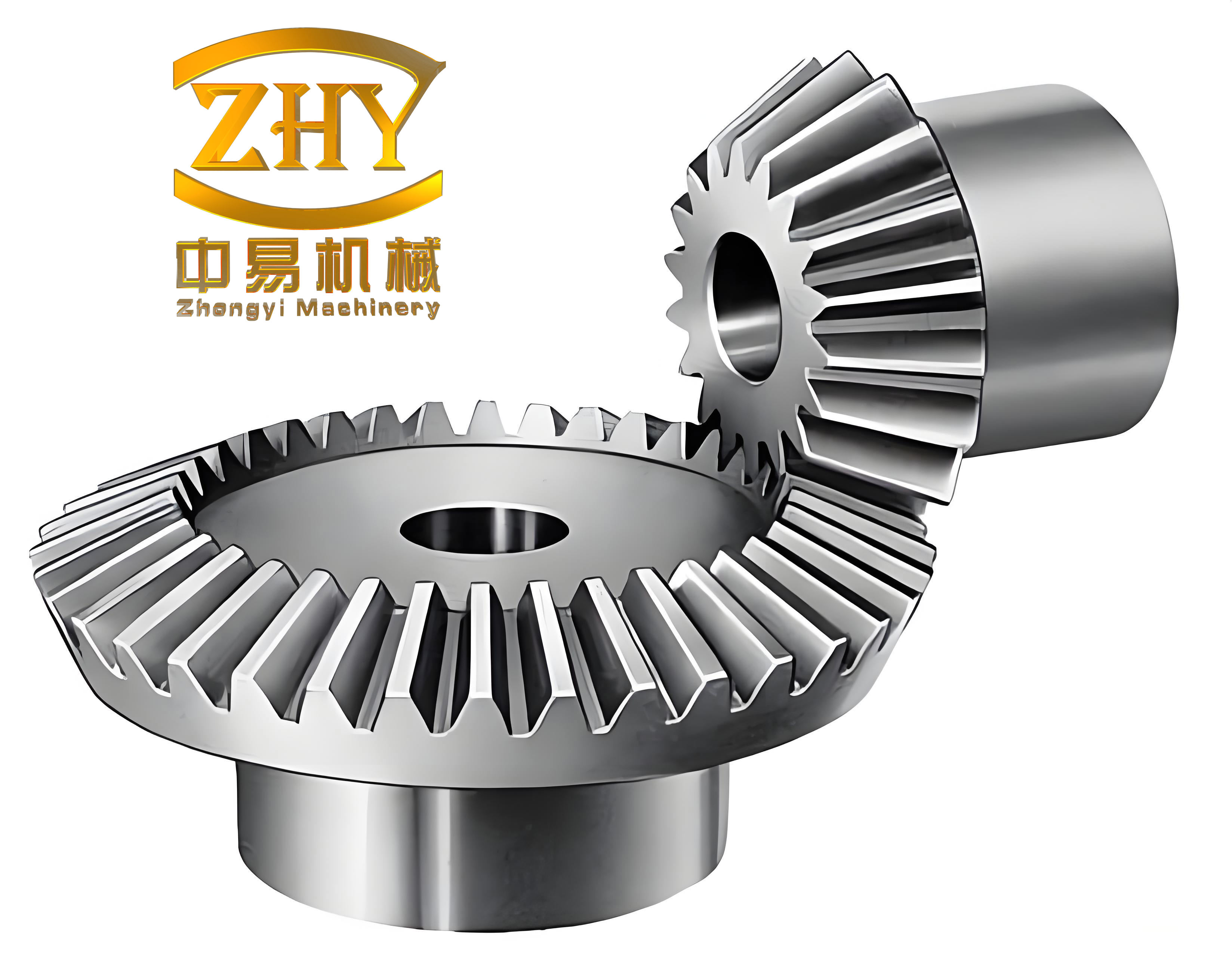
Next, I derive the relative sliding and rolling velocities. The tangential velocities of the two flanks at the contact point are \(R_1 \omega_1\) and \(R_2 \omega_2\). Their normal components are equal, so the sliding velocity is
$$ V_S(\phi,r) = R_1 \omega_1 – R_2 \omega_2 $$
and the rolling velocity is
$$ V_R(\phi,r) = R_1 \omega_1 + R_2 \omega_2 $$
Substituting the expressions for \(R_1\) and \(R_2\), and expressing angular velocity in terms of the rotational speed \(n_1\) of the driving straight bevel gear, I obtain
$$ V_S(\phi,r) = \frac{\pi \cos \alpha’}{30 \cos \delta_1} n_1 r \left[ \left(1+\frac{1}{i}\right) \tan \phi – \left(1+\frac{1}{i}\right) \tan \alpha’ \right] \times 10^{-3} $$
$$ V_R(\phi,r) = \frac{\pi \cos \alpha’}{30 \cos \delta_1} n_1 r \left[ \left(1-\frac{1}{i}\right) \tan \phi + \left(1+\frac{1}{i}\right) \tan \alpha’ \right] \times 10^{-3} $$
These velocities vary along the tooth width (through \(r\)) and along the line of action (through \(\phi\)). As expected, the sliding velocity is zero at the pitch point where \(\phi = \alpha’\). The rolling velocity is always positive and reaches its maximum at the large end of the tooth.
The load distribution on the tooth flank is another critical factor. I assume that the distributed load along the contact line varies linearly from the large end to the small end. The tooth width is denoted by \(B\). Let \(r_1\) and \(r’_1\) be the large-end and small-end pitch radii, respectively. The distributed load per unit width \(w(r)\) is proportional to the penetration depth, which in turn is related to the elastic deformation. For a single tooth pair in contact, the distributed load is
$$ w(r) = \frac{3 T \sin \delta_1}{(r_1^3 – r’^3_1) \cos \alpha’} r $$
where \(T\) is the input torque. This linear variation reflects the taper of the straight bevel gear tooth. When multiple tooth pairs share the load, the load sharing coefficient \(k_\alpha\) must be considered. For a typical contact ratio between 1 and 2, there are double-tooth and single-tooth contact regions. The load sharing coefficients at the start and end of double contact are \(k_{\alpha B1} = k_{\alpha B2} = 9/20\), while at the transition points they are \(k_{\alpha C} = k_{\alpha D} = 11/20\). The actual distributed load at any pressure angle \(\phi\) is then
$$ w(\phi,r) = \begin{cases}
k_{B1C} (\phi – \alpha_{B1}) + \frac{9}{20} w(r), & \text{double contact} \\
w(r), & \text{single contact} \\
k_{DB2} (\alpha_{B2} – \phi) + \frac{9}{20} w(r), & \text{double contact}
\end{cases} $$
where \(k_{B1C} = w(r) / [10(\alpha_C – \alpha_{B1})]\), \(k_{DB2} = w(r) / [10(\alpha_{B2} – \alpha_D)]\), and \(\alpha_{B1}, \alpha_C, \alpha_D, \alpha_{B2}\) are the pressure angles at the key points on the line of action. These angles are determined by the equivalent gear geometry and are given in the simulation section.
The lubrication state is determined by the film thickness ratio. I use the Dowson-Higginson formula to calculate the minimum oil film thickness:
$$ h_{\min}(\phi,r) = \frac{2.65 \alpha^{0.54} (\eta_0 U)^{0.7} R(\phi,r)^{0.43}}{E’^{0.03} w(\phi,r)^{0.13}} $$
where \(\alpha\) is the pressure-viscosity coefficient, \(\eta_0\) is the dynamic viscosity at atmospheric pressure, \(U\) is the entrainment velocity, and \(E’\) is the effective elastic modulus. The entrainment velocity is
$$ U = \frac{R_{v1} \omega_1 + R_{v2} \omega_2}{2} \times 10^{-3} = \frac{\pi}{60} n_1 r_{vb1} \left[ \left(1+\frac{1}{i}\right) \tan \alpha’ + \left(1-\frac{1}{i}\right) \tan \phi \right] $$
The average film thickness is \(h_{av} = 4 h_{\min} / 3\). The film thickness ratio \(\lambda\) is defined as
$$ \lambda = \frac{h_{av}}{\sqrt{\sigma_1^2 + \sigma_2^2}} $$
where \(\sigma_1\) and \(\sigma_2\) are the RMS surface roughness of the two gear flanks. Based on \(\lambda\), the lubrication state is classified as boundary lubrication (\(\lambda \leq 0.9\)), mixed lubrication (\(0.9 < \lambda < 3\)), or elastohydrodynamic lubrication (\(\lambda \geq 3\)). This classification is summarized in Table 1.
| Lubrication regime | Film thickness ratio \(\lambda\) | Key characteristics |
|---|---|---|
| Boundary | \(\lambda \leq 0.9\) | Direct asperity contact, load carried by peaks |
| Mixed | \(0.9 < \lambda < 3\) | Partial oil film, asperities and fluid share load |
| Elastohydrodynamic | \(\lambda \geq 3\) | Full film, elastic deformation and viscosity effects |
For each lubrication regime, I adopt a different friction coefficient model. In boundary lubrication, the friction coefficient is assumed constant: \(f_b = 0.15\). In elastohydrodynamic lubrication, I use the Benedict-Kelley empirical formula:
$$ f_e(\phi,r) = 0.0127 \left( \frac{50}{50 – 39.37 \delta} \right) \lg \left( \frac{29.66 w(\phi,r)}{\rho V_S(\phi,r) V_R^2(\phi,r)} \right) $$
where \(\delta\) is the surface roughness in micrometers and \(\rho\) is the lubricant viscosity in Pa·s. For mixed lubrication, the friction coefficient is a weighted combination of boundary and EHL values:
$$ f_m(\phi,r) = f_\lambda^{1.2} f_e + (1 – f_\lambda) f_b $$
where the load-carrying ratio of the full film is
$$ f_\lambda = \frac{1.21 \lambda^{0.64}}{1 + 0.37 \lambda^{1.26}} $$
This mixed lubrication model smoothly transitions between the two limiting regimes and is well suited for the complex lubrication states encountered in straight bevel gears.
The instantaneous sliding friction power loss at any contact point is
$$ P_S(\phi,r) = f(\phi,r) F_n(\phi,r) V_S(\phi,r) \times 10^{-3} $$
where \(F_n(\phi,r)\) is the normal load per unit width, which can be obtained by integrating the distributed load along the contact line. Since the distributed load varies with \(r\), the total normal load on a single tooth pair is
$$ F_n = \int_{r’_1}^{r_1} w(r) \, dB = \frac{\pi \theta}{4 \sin^2 \delta_1} (r_1^2 – r’^2_1) E’ $$
with \(\theta\) being the angular deformation of the contact line. The rolling friction power loss is modeled using the Crook formula:
$$ P_R(\phi,r) = 90 h(\phi,r) V_R(\phi,r) b \times 10^{-3} $$
where \(b\) is the contact width and \(h(\phi,r)\) is the elastohydrodynamic film thickness. To obtain the average power loss over one meshing cycle, I perform a double integration over the pressure angle and the pitch radius. For sliding power loss, the integration is carried out separately for the three contact regions: double contact near the start, single contact in the middle, and double contact near the end. The total sliding power loss is
$$ P_{S,\text{total}} = \frac{(\alpha_{B2} – \alpha_{B1}) Z_1}{2\pi} \frac{1}{\alpha_{B2} – \alpha_{B1}} \sum_{i=1}^{3} \sum_{\phi,r} \left[ f(\phi,r) F_n(\phi,r) V_S(\phi,r) \times 10^{-3} \right] $$
where \(Z_1\) is the number of teeth on the driving straight bevel gear. Similarly, the total rolling power loss is
$$ P_{R,\text{total}} = \frac{(\alpha_{B2} – \alpha_{B1}) Z_1}{2\pi} \frac{1}{\alpha_{B2} – \alpha_{B1}} \sum_{i=1}^{3} \int_{r’_1}^{r_1} \int_{\alpha_i}^{\beta_i} 90 h(\phi,r) V_R(\phi,r) \times 10^{-3} \, d\phi \, dr $$
The total meshing power loss is the sum of the sliding and rolling contributions:
$$ P_t = P_{S,\text{total}} + P_{R,\text{total}} $$
Finally, the meshing efficiency of the straight bevel gears is
$$ \eta = \frac{P – P_t}{P} $$
where \(P\) is the input power. This efficiency accounts for both sliding and rolling friction losses under the actual lubrication state.
To validate the model, I performed a simulation study using a representative pair of straight bevel gears. The main parameters are listed in Table 2. The driving gear has 24 teeth, the driven gear has 48 teeth, and the module is 5 mm. The pressure angle is 25°, the face width is 100 mm, and the input torque is 200 N·m. The rotational speed of the driving gear is 3000 rpm. The surface roughness is 0.4 μm RMS, the effective elastic modulus is \(2.3 \times 10^{11}\) N/m², the lubricant viscosity at 60°C is 0.075 Pa·s, and the pressure-viscosity coefficient is \(2.2 \times 10^{-8}\) m²/N.
| Parameter | Value |
|---|---|
| Number of teeth (driving/driven) | 24 / 48 |
| Module | 5 mm |
| Pressure angle | 25° |
| Pitch diameter (driving) | 121 mm |
| Face width | 100 mm |
| Input torque | 200 N·m |
| Driving speed | 3000 rpm |
| Surface roughness (RMS) | 0.4 μm |
| Effective elastic modulus | \(2.3 \times 10^{11}\) N/m² |
| Lubricant viscosity (60°C) | 0.075 Pa·s |
| Pressure-viscosity coefficient | \(2.2 \times 10^{-8}\) m²/N |
From the gear geometry, I calculated the key pressure angles along the line of action. These are listed in Table 3. The theoretical center distance is 90.85 mm, and the actual center distance is 90.86 mm. The normal pitch is 11.2466 mm, and the mesh angle is 0.4363 rad. The pressure angles at the start and end of contact, and at the transition points, are \(\alpha_{B1}=0.2723\) rad, \(\alpha_C=0.3829\) rad, \(\alpha_D=0.4743\) rad, and \(\alpha_{B2}=0.5671\) rad.
| Parameter | Value |
|---|---|
| Theoretical center distance | 90.85 mm |
| Actual center distance | 90.86 mm |
| Normal pitch | 11.2466 mm |
| Mesh angle | 0.4363 rad |
| \(\alpha_{B1}\) | 0.2723 rad |
| \(\alpha_C\) | 0.3829 rad |
| \(\alpha_D\) | 0.4743 rad |
| \(\alpha_{B2}\) | 0.5671 rad |
The simulation results reveal several important trends. First, the relative sliding velocity increases from the small end to the large end of the tooth, and its minimum occurs near the pitch point. The rolling velocity also increases from the small end to the large end, but it is less sensitive to the pressure angle. These trends are consistent with the kinematics of straight bevel gears. Second, the distributed load decreases from the large end to the small end, but the decrease is not perfectly linear; it follows a slightly parabolic shape due to the taper. The oil film thickness increases from the small end to the large end, and it is thinner in the single-tooth contact region because the load is higher there. Third, the film thickness ratio \(\lambda\) ranges from 0.9124 to 4.8565, indicating that the lubrication state is a combination of mixed and elastohydrodynamic lubrication. Boundary lubrication does not occur under these conditions. The elastohydrodynamic region is concentrated near the large end, especially near the end of contact, while the mixed lubrication region dominates near the small end.
The friction coefficient under mixed lubrication is shown in Table 4 for representative points. Near the large end and at high rolling velocities, the friction coefficient is lower because the EHL film is thicker. Near the small end and at low rolling velocities, the friction coefficient approaches the boundary value. The sliding friction power loss increases from the small end to the large end, and it is zero at the pitch point. The rolling friction power loss also increases from the small end to the large end, with its maximum at the large end near the end of contact. The total power loss is dominated by sliding friction, especially in the mixed lubrication regime.
| Location | \(\lambda\) | \(f_m\) | Dominant regime |
|---|---|---|---|
| Small end, start of contact | 1.12 | 0.098 | Mixed |
| Mid-width, pitch point | 2.35 | 0.072 | Mixed |
| Large end, end of contact | 4.21 | 0.041 | EHL |
To evaluate the overall performance, I computed the total power loss and efficiency for different input speeds. The results are summarized in Table 5. As the input speed increases from about 600 rpm to 3000 rpm, the total power loss increases, but the efficiency also increases slightly because the EHL film becomes thicker and the friction coefficient decreases. At 598.2 rpm, the theoretical efficiency is 90.63%, while the experimental efficiency is 89.47%. At higher speeds, the theoretical efficiency reaches 91.52%, and the experimental value is 90.78%. The difference between theory and experiment is mainly due to noise, vibration, and other unmodeled losses. Nevertheless, the trend is consistent, and the maximum deviation is within acceptable limits.
| Speed (rpm) | Theoretical power loss (kW) | Experimental power loss (kW) | Theoretical efficiency (%) | Experimental efficiency (%) |
|---|---|---|---|---|
| 598.2 | 0.037 | 0.053 | 90.63 | 89.47 |
| 1200 | 0.082 | 0.101 | 90.95 | 89.82 |
| 1800 | 0.134 | 0.158 | 91.18 | 90.12 |
| 2400 | 0.195 | 0.224 | 91.36 | 90.45 |
| 3000 | 0.263 | 0.298 | 91.52 | 90.78 |
The load distribution along the contact line was also compared with finite element results. A linear distribution curve with a slope of 20.6 was reported in earlier studies. Using my method, the slope of the single-tooth load distribution is 18.4. This is the same order of magnitude, which confirms that my simplified load distribution is reasonable and provides a good approximation for straight bevel gears. The small discrepancy is due to the boundary effects at the tooth ends, which are neglected in my analytical model. For more accurate results, a three-dimensional finite element contact analysis could be coupled with my lubrication and friction models.
Several conclusions can be drawn from this study. First, the equivalent gear principle is effective for analyzing the meshing efficiency of straight bevel gears. By transforming the straight bevel gears into equivalent spur gears, I can apply well-established lubrication and friction models while accounting for the tapered tooth geometry through the load distribution and kinematic parameters. Second, the lubrication state of straight bevel gears is highly non-uniform. Under typical operating conditions, mixed and elastohydrodynamic lubrication coexist, and the transition depends on the local film thickness ratio. Third, the sliding friction power loss is the dominant contributor to the total power loss, especially in the mixed lubrication regime. Rolling friction is smaller but not negligible. Fourth, the total meshing efficiency increases with speed because the EHL film becomes thicker and the friction coefficient decreases. The theoretical model predicts efficiencies in the range of 90.6% to 91.5%, which are close to experimental measurements.
My model has some limitations. The load distribution is assumed to be linear along the tooth width, and the boundary effects at the tooth ends are ignored. In reality, the load distribution may be more complex, especially near the edges. Also, the friction coefficient models are empirical and may not capture all the details of mixed lubrication. Future work could incorporate a more detailed contact analysis and a transient thermal model to account for temperature effects on lubricant viscosity. Despite these limitations, the proposed model provides a useful tool for predicting the meshing efficiency of straight bevel gears under complex lubrication states. It can be used for thermal analysis, lubrication system design, and efficiency optimization of straight bevel gear transmissions.
In summary, I have established a comprehensive analytical model for the meshing efficiency of straight bevel gears. The model integrates the equivalent gear principle, time-varying load distribution, film thickness calculation, and regime-specific friction coefficient models. The double integration over the mesh cycle allows accurate prediction of sliding and rolling power losses. The simulation results demonstrate that the model can capture the key trends and provide reasonable quantitative agreement with experiments. This work contributes to a better understanding of the tribological behavior of straight bevel gears and offers a practical method for efficiency evaluation in engineering design.