
The pursuit of precision, compactness, and high-performance motion control has consistently driven innovation in mechanical transmission systems. Among the various solutions available, harmonic drive gears stand out due to their unique operating principle and exceptional characteristics. A harmonic drive gear is a specialized mechanical gear system renowned for its ability to provide high reduction ratios within an extremely compact package, alongside features such as high positional accuracy, minimal backlash, and quiet operation. The fundamental operation relies on the controlled elastic deformation of a critical component, making its analysis distinct from that of conventional rigid-body gear systems. This article delves into a detailed investigation of the dynamic characteristics of the core component in a harmonic drive gear—the flexspline—using advanced finite element methods, with a particular focus on modal analysis to ensure operational reliability and avoid detrimental resonant conditions.
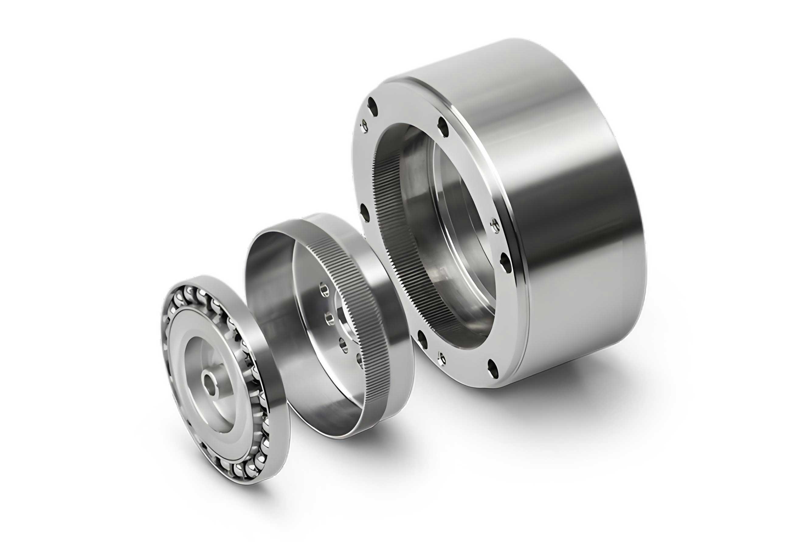
The operational excellence of a harmonic drive gear is achieved through the synergistic interaction of three primary components: a rigid circular spline, a flexible spline (flexspline), and an elliptical or cam-type wave generator. The wave generator, typically an elliptical bearing assembly, is inserted into the flexspline, causing its initially circular rim to deform into an elliptical shape. This deformation engages the teeth of the flexspline with those of the rigid circular spline at two diametrically opposite regions. As the wave generator rotates, the points of engagement travel, creating a relative motion between the flexspline and the circular spline. Because the flexspline has fewer teeth (typically by 2) than the circular spline, each full rotation of the wave generator results in a very small relative rotation between the two splines, yielding a high gear reduction ratio. The performance and longevity of the entire harmonic drive gear assembly are inextricably linked to the structural integrity of the flexspline, which undergoes cyclic elastic deformation during every operational cycle.
Within the harmonic drive gear, the flexspline serves as the torque-transmitting element that is subjected to continuous alternating stresses. Its primary failure mode is fatigue fracture originating from stress concentrations, often at the fillet region of the teeth or the junction between the thin-walled cylinder and the diaphragm or flange. Therefore, a comprehensive understanding of its static and dynamic behavior is paramount for designers. While static stress analysis under load is crucial for determining ultimate strength, dynamic analysis, specifically modal analysis, is essential for predicting vibrational behavior. If the excitation frequency from the rotating wave generator or external loads coincides with a natural frequency of the flexspline, resonance can occur. Resonance leads to amplified vibrational amplitudes, drastically accelerating fatigue damage, increasing noise, and potentially causing catastrophic failure. Hence, calculating the natural frequencies and corresponding mode shapes of the flexspline is a critical step in the design validation process for any harmonic drive gear.
Fundamental Mechanics and the Need for Dynamic Analysis
The flexspline in a harmonic drive gear is a complex, thin-walled cylindrical structure with external gear teeth. Its dynamic behavior can be modeled by the general equation of motion for a continuous elastic body. For undamped free vibration, which forms the basis of modal analysis, the equation is derived from elasticity theory and Newton’s second law. The governing differential equation for the displacement field \(\mathbf{u}(\mathbf{x}, t)\) within the flexspline volume \(V\) is given by:
$$
\nabla \cdot \boldsymbol{\sigma} + \mathbf{f} = \rho \frac{\partial^2 \mathbf{u}}{\partial t^2}
$$
where \(\boldsymbol{\sigma}\) is the Cauchy stress tensor, \(\mathbf{f}\) is the body force vector (often negligible in modal analysis), and \(\rho\) is the material density. For a linear elastic material obeying Hooke’s Law, the stress is related to the strain \(\boldsymbol{\varepsilon}\) by the fourth-order elasticity tensor \(\mathbf{C}\):
$$
\boldsymbol{\sigma} = \mathbf{C} : \boldsymbol{\varepsilon} \quad \text{and} \quad \boldsymbol{\varepsilon} = \frac{1}{2}[\nabla \mathbf{u} + (\nabla \mathbf{u})^T]
$$
Assuming harmonic motion for free vibration, the displacement can be separated into spatial and temporal components: \(\mathbf{u}(\mathbf{x}, t) = \mathbf{U}(\mathbf{x}) e^{i \omega t}\), where \(\mathbf{U}(\mathbf{x})\) is the mode shape vector and \(\omega\) is the circular natural frequency in radians per second. Substituting this into the governing equation and neglecting body forces leads to the classical eigenvalue problem:
$$
\nabla \cdot (\mathbf{C} : \nabla \mathbf{U}) + \rho \omega^2 \mathbf{U} = 0
$$
Solving this partial differential equation analytically for a complex geometry like a geared flexspline is virtually impossible. This is where the Finite Element Method (FEM) provides a powerful numerical approach. The FEM discretizes the continuous flexspline geometry into a finite number of small, simple elements interconnected at nodes. The continuous eigenvalue problem is thus approximated by a discrete generalized eigenvalue problem of the form:
$$
[\mathbf{K}] \{\mathbf{\Phi}\}_i = \omega_i^2 [\mathbf{M}] \{\mathbf{\Phi}\}_i
$$
where \([\mathbf{K}]\) is the global stiffness matrix assembled from element stiffness matrices, \([\mathbf{M}]\) is the global consistent or lumped mass matrix, \(\omega_i\) is the \(i\)-th natural frequency, and \(\{\mathbf{\Phi}\}_i\) is the corresponding eigenvector representing the discretized mode shape. The solution to this matrix equation yields the natural frequencies \(f_i = \omega_i / (2\pi)\) and mode shapes of the discretized structure. For a harmonic drive gear designer, the lower-order natural frequencies (typically the first 10-20 modes) are of primary interest, as they are most likely to be excited by operational forces.
Finite Element Modeling of the Cylindrical Flexspline
Accurate modal analysis of a harmonic drive gear flexspline hinges on the creation of a high-fidelity finite element model. This process involves several key steps: geometric modeling, material property definition, element selection, and mesh generation. The following sections detail this procedure.
Geometric Definition and Simplifications
This study focuses on a common cylindrical cup-type flexspline. The major geometric parameters required for modeling are derived from standard gear design equations and specific dimensional constraints of the harmonic drive gear assembly. While a perfect model would include every minute detail, intelligent simplifications are necessary to make the finite element analysis computationally tractable without significantly compromising result accuracy. Features such as small fillets at the tooth root, minor chamfers on the flange, and very small surface irregularities have a negligible effect on global natural frequencies, though they are critical for local stress concentration analysis. Therefore, these features are often suppressed during the geometry creation phase for modal analysis.
The primary dimensions are defined by the gear parameters and the cup geometry. A representative set of parameters for a cylindrical flexspline in a harmonic drive gear is summarized in the table below. These parameters are used to generate a three-dimensional solid model, typically using parametric CAD software like Pro/ENGINEER (Creo), SOLIDWORKS, or similar, which allows for easy modification and design iteration.
| Parameter Category | Symbol | Value | Unit | |
|---|---|---|---|---|
| Gear Parameters | Module | \(m\) | 0.5 | mm |
| Number of Teeth | \(z\) | 429 | – | |
| Pressure Angle | \(\alpha\) | 20 | ° | |
| Addendum Coefficient | \(h_a^*\) | 1.0 | – | |
| Dedendum/Clearance Coefficient | \(c^*\) | 0.25 | – | |
| Derived Gear Dimensions | Pitch Diameter | \(d\) | \(m \times z = 214.5\) | mm |
| Base Circle Diameter | \(d_b\) | \(d \cdot \cos(\alpha)\) | ~200.38 mm | |
| Addendum Diameter | \(d_a\) | \(d + 2m \cdot h_a^*\) | 215.5 mm | |
| Dedendum Diameter | \(d_f\) | \(d – 2m \cdot (h_a^* + c^*)\) | 213.0 mm | |
| Tooth Width | \(b_r\) | 40 | mm | |
| Cup Geometry | Cylinder Length | \(L\) | 180 | mm |
| Cylinder Wall Thickness | \(\delta_1\) | 3.6 | mm | |
| Gear Rim Wall Thickness | \(\delta\) | 6.0 | mm |
Material Properties and Element Selection
The choice of material for the flexspline in a harmonic drive gear is critical, requiring high fatigue strength, good elastic properties, and manufacturability. A common choice is alloy steel such as 35CrMnSiA. The linear elastic material properties essential for modal analysis are the Young’s Modulus (E), Poisson’s Ratio (ν), and Density (ρ). These are defined as follows for the subsequent finite element analysis:
| Material Property | Symbol | Value | Unit |
|---|---|---|---|
| Young’s Modulus | \(E\) | 196 | GPa |
| Poisson’s Ratio | \(\nu\) | 0.28 | – |
| Density | \(\rho\) | 7850 | kg/m³ |
For the finite element discretization, a robust 3D solid element is required. ANSYS provides the SOLID185 element, which is well-suited for this application. It is defined by eight nodes, each having three translational degrees of freedom (UX, UY, UZ). This element can model complex stress states, large deflections, and is appropriate for modal analysis as it contributes accurately to both the stiffness and mass matrices. The use of a 3D solid element, as opposed to shell elements, is advantageous for capturing the three-dimensional mode shapes that involve deformation through the thickness of the flexspline wall, especially in the geared region.
Mesh Generation Strategy
The meshing process is a crucial step that influences the accuracy and convergence of the modal analysis results. The flexspline geometry presents a challenge due to the significant disparity in feature sizes: the thin walls versus the finely spaced gear teeth. A global uniform mesh would be prohibitively dense and computationally expensive. Therefore, a partitioned approach is adopted. The model is divided into logical sections: the smooth thin-walled cylinder and the thicker geared rim. Different mesh sizing controls are applied to each section.
The gear teeth require a sufficiently fine mesh to capture their geometry and the local stiffness correctly, but the mesh in the cylinder can be coarser. A transition zone ensures mesh compatibility. A swept or mapped meshing technique is often employed for the cylindrical section to create a regular grid of hexahedral elements, which generally provide better accuracy than tetrahedral elements. The geared section may utilize a free tetrahedral mesh or a controlled hex-dominant mesh. The final meshed model should be checked for element quality metrics such as aspect ratio, skewness, and Jacobian to ensure numerical stability. Contact elements are not required for a free-vibration modal analysis, as the analysis is performed on a single, continuous component without external constraints from the wave generator or circular spline (these would be considered in a subsequent prestressed modal analysis).
Theory and Execution of Modal Analysis
Modal analysis, as applied to the harmonic drive gear flexspline, is the process of determining its inherent vibration characteristics—the natural frequencies and mode shapes. These are intrinsic properties of the structure, determined by its mass distribution, stiffness distribution, and boundary conditions. In a free-free modal analysis, which is commonly performed first, the component is considered unconstrained in space. This simulates the condition of the flexspline before assembly or its dynamic behavior when isolation from the housing is considered. However, for a more realistic operational scenario, a constrained modal analysis with boundary conditions representing the mounting flange (e.g., all degrees of freedom fixed at the flange face) is also essential.
The discrete generalized eigenvalue problem solved by the FEM, \([\mathbf{K}]\{\mathbf{\Phi}\}_i = \omega_i^2 [\mathbf{M}]\{\mathbf{\Phi}\}_i\), is at the core of the solution. Numerical algorithms, such as the Block Lanczos or Subspace iteration method available in ANSYS, are used to extract a subset of eigenvalues (\(\lambda_i = \omega_i^2\)) and eigenvectors \(\{\mathbf{\Phi}\}_i\). The Block Lanczos method is highly efficient for extracting a large number of modes from large-scale models, making it suitable for the detailed flexspline model with many degrees of freedom.
The setup for the modal analysis involves specifying the analysis type as “Modal,” selecting the appropriate eigenvalue solver and options, and defining the number of modes to extract. For a harmonic drive gear application, it is crucial to extract enough modes to cover the frequency range of potential excitation sources. The maximum operational speed of the wave generator defines the primary excitation frequency \(f_{ex}\):
$$
f_{ex} = \frac{N}{60}
$$
where \(N\) is the rotational speed of the wave generator in RPM. Harmonics of this frequency (\(2f_{ex}, 3f_{ex}\), etc.) may also be present due to nonlinearities or imperfections. Therefore, the extracted frequency range should extend well beyond the highest significant harmonic of \(f_{ex}\). A common practice is to request the first 10 to 20 modes to ensure a comprehensive view of the low to mid-frequency dynamic behavior of the harmonic drive gear flexspline.
Results and Discussion of Modal Characteristics
Upon solving the eigenvalue problem, the finite element software outputs the natural frequencies and allows for visualization of the corresponding mode shapes. The natural frequencies are typically listed in ascending order. The mode shapes reveal the pattern of deformation associated with each frequency. For a cylindrical structure like the flexspline, the lower-order modes often involve gross bending, ovaling (2-nodal diameter), triangulation (3-nodal diameter), and higher-order shell-type modes, combined with axial and torsional deformation. The presence of the gear teeth locally stiffens the rim, which can slightly alter the frequencies compared to a plain cylinder but does not change the fundamental nature of the modes.
The following table presents a hypothetical but representative set of results for the first ten natural frequencies of a cylindrical cup-type flexspline from a free-free modal analysis, as might be generated in ANSYS. The “Mode Description” attempts to characterize the dominant deformation pattern observed in the visualization.
| Mode Number | Natural Frequency, \(f_n\) (Hz) | Dominant Mode Shape Description |
|---|---|---|
| 1 | 412.5 | First Bending (Beam-like) |
| 2 | 413.1 | First Bending (Orthogonal direction) |
| 3 | 1025.7 | First Torsion |
| 4 | 1678.3 | Second Bending |
| 5 | 1680.0 | Second Bending (Orthogonal) |
| 6 | 2450.2 | Cylinder Ovaling (2-nodal diameter) |
| 7 | 3321.8 | Combined Axial/Bending (High displacement) |
| 8 | 3330.5 | Combined Axial/Bending (High displacement, orthogonal) |
| 9 | 4100.4 | Cylinder Triangulation (3-nodal diameter) |
| 10 | 4987.6 | Second Torsion / Shell mode |
The most critical step for the harmonic drive gear designer is the resonance avoidance check. This involves comparing the extracted natural frequencies \(f_n\) with the system’s excitation frequencies \(f_{ex}\). A standard rule of thumb is to maintain a separation margin, often 15-20%, to account for uncertainties in modeling, material properties, and boundary conditions. The condition to avoid is:
$$
f_{ex} \approx f_n \quad \text{or} \quad k \cdot f_{ex} \approx f_n \quad (k=1,2,3,…)
$$
If the wave generator speed is, for example, 3000 RPM, then \(f_{ex} = 50\) Hz. Even its 10th harmonic (500 Hz) is well below the first bending mode (~413 Hz in this example, but note: in a constrained analysis the first mode would be much higher). However, if the harmonic drive gear were used in a high-speed application with a wave generator speed of 24,000 RPM (\(f_{ex} = 400\) Hz), the first bending mode at 412.5 Hz would pose a severe resonance risk, necessitating a design change. Modes 7 and 8 in the table above, with frequencies around 3325 Hz, are noted to have particularly high displacement magnitudes in the visualization. This indicates these modes have a high dynamic compliance (low modal stiffness), meaning if excited, they would produce large vibration amplitudes. The operational speed of the harmonic drive gear must be meticulously planned to ensure neither the fundamental nor any major harmonic coincides with these sensitive frequencies.
Parametric Studies and Design Implications
Finite element modal analysis is not merely a verification tool but a powerful guide for optimizing the harmonic drive gear flexspline design. By parametrically varying key dimensions and observing the shift in natural frequencies, designers can tune the dynamic response. The natural frequency of a simplified beam or cylindrical shell is governed by relations of the form:
$$
f_n \propto \frac{1}{L^2} \sqrt{\frac{E I}{\rho A}} \quad \text{(for bending)} \quad \text{or} \quad f_n \propto \frac{1}{R} \sqrt{\frac{E}{\rho}} \quad \text{(for shell modes)}
$$
where \(L\) is length, \(R\) is radius, \(I\) is area moment of inertia, \(A\) is cross-sectional area, \(E\) is Young’s modulus, and \(\rho\) is density. This implies that:
- Wall Thickness (\(\delta, \delta_1\)): Increasing the wall thickness raises the moment of inertia \(I\), thereby increasing stiffness more significantly than mass, leading to higher natural frequencies. This is an effective way to push critical modes out of an excitation frequency range.
- Cylinder Length (\(L\)): Reducing the length of the flexspline cup has a very strong effect on increasing bending frequencies (inverse square relationship). This is often a primary driver in choosing shorter “pancake” style harmonic drive gear designs for higher dynamic performance.
- Material Properties: Using a material with a higher specific stiffness \(E/\rho\) (e.g., titanium alloys or certain advanced composites) can raise all natural frequencies proportionally.
- Flange/Diaphragm Design: The stiffness of the connection between the cylindrical barrel and the mounting flange profoundly affects the boundary conditions. A stiffer diaphragm raises the lower-frequency constrained modes.
A systematic parametric study involves creating multiple FE models, varying one parameter at a time within a realistic range, and performing modal analysis on each. The results can be plotted to create sensitivity charts, showing which design parameters have the greatest leverage on the dynamic behavior of the harmonic drive gear flexspline. This data-driven approach allows engineers to make informed trade-offs between weight, stiffness, stress, and dynamic performance.
Conclusion
Modal analysis using the Finite Element Method, as exemplified through ANSYS, is an indispensable component in the modern design and validation process for harmonic drive gears. The flexspline, being the cyclically deforming heart of the system, must be designed not only for static strength but also for dynamic integrity. By building a detailed finite element model that accurately represents the geometry and material of the cylindrical flexspline, engineers can extract its fundamental natural frequencies and mode shapes. This information is critical for conducting a resonance avoidance check, ensuring that the operational excitation frequencies from the wave generator and driven load do not coincide with any of the flexspline’s resonant modes, particularly those with high modal displacement. The analysis reveals that modes involving combined axial and bending deformations can be especially sensitive. Furthermore, the FE model serves as a platform for parametric optimization, enabling designers to adjust dimensions like wall thickness and cup length to shift the natural frequency spectrum and enhance the overall robustness and reliability of the harmonic drive gear. In summary, a thorough dynamic analysis grounded in finite element simulation is paramount for advancing the performance envelope, lifespan, and operational safety of high-precision harmonic drive gear systems.