
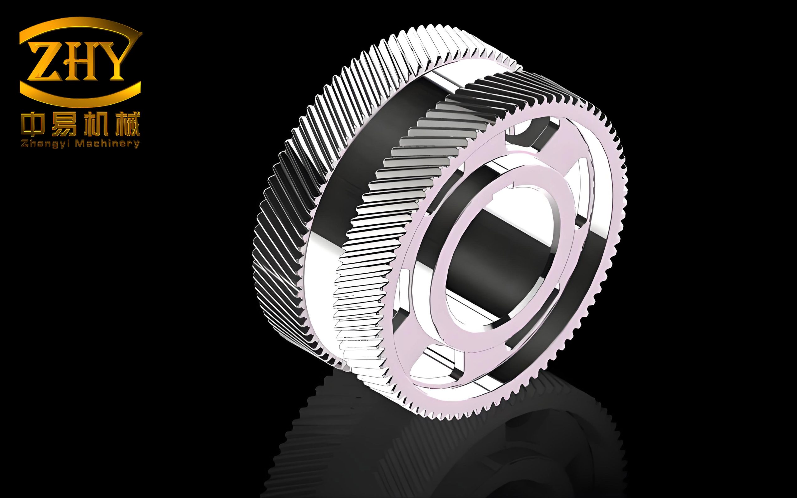
Modern mechanical equipment is rapidly advancing toward heavy-load, high-precision applications, demanding ever-improving performance from mechanical transmission systems. Herringbone gears combine the advantages of both spur and helical gear drives—they provide stable and reliable transmission, low impact and noise, while eliminating the axial thrust that helical gears impose on shafts, which is especially critical under heavy-load conditions where large axial forces could degrade transmission performance. As a result, herringbone gears are widely used in marine propulsion, aerospace, and industrial machinery.
However, manufacturing errors are inevitable in herringbone gear production. Since a herringbone gear is formed by combining two helical gear halves with opposite helix directions, its structure is inherently more complex than that of standard helical gears. Herringbone gears exhibit alignment errors at the central plane, and both the left-hand and right-hand helical tooth flank errors must be considered. These error sources collectively induce transmission errors in herringbone gear systems, affecting the stability and accuracy of the entire machine. In this thesis, a slice discretization approach is employed to establish a transmission accuracy model for herringbone gears. Based on the measurement and equivalent representation of various manufacturing errors, the influence of these errors on system transmission accuracy is investigated. The transmission performance of herringbone gear systems is analyzed and evaluated.
1 Introduction
Gear transmission systems are indispensable for power transmission in mechanical equipment. Among all gear types, herringbone gears—also known as double-helical gears—offer exceptional load-carrying capacity, smooth meshing, high efficiency, and compact structuring. They inherently balance axial forces because of their symmetric helix arrangement, eliminating the need for thrust bearings while preserving the smooth engagement characteristics of helical gears. This makes them the preferred choice for high-speed, heavy-load applications such as marine main gearboxes, helicopter transmissions, and large-scale industrial reducers.
The transmission error (TE) of gear systems is a fundamental performance metric that directly influences vibration, noise, and positioning accuracy. Transmission error is defined as the difference between the actual angular position of the driven gear and its theoretical angular position. Manufacturing errors—such as tooth profile deviation, helix deviation, pitch deviation, and the unique alignment error of herringbone gears—perturb the ideal conjugate action of gear pairs, resulting in periodic and non-periodic transmission error components. The accurate modeling and prediction of transmission error under realistic manufacturing deviations are therefore of paramount importance.
In the past decades, researchers have developed various models for gear transmission accuracy. Early models treated contact teeth as rigid bodies with spring-damper elements inserted at the contact to simulate inter-tooth forces. Smith pointed out that both manufacturing errors and assembly errors contribute to the integrated transmission error of gear systems. Mark derived Fourier series coefficient expressions for the static transmission error of helical gear pairs. Driot and Perret-Liaudet utilized finite element analysis to obtain static transmission errors at varying load levels. Lin applied finite element methods to investigate the effects of machining errors, assembly errors, and tooth modifications on static transmission error. Yuan and colleagues developed a generalized loaded static transmission error model accounting for elastic deformation of gear pairs. More recent studies by Guo and Fang incorporated measured manufacturing errors into dynamic models of spiral bevel gears, analyzing time-domain and frequency-domain responses. For herringbone gears, however, existing models often oversimplify the double-helix structure or fail to incorporate realistic measured error distributions across both flanks.
This thesis aims to bridge this gap by establishing a slice-based transmission accuracy model for herringbone gears. The approach combines the computational efficiency of analytical methods with the capability to handle spatial tooth flank error variations. The major contributions include: (1) systematic fitting and equivalent representation of measured manufacturing errors for herringbone gears; (2) establishment of a pair-type herringbone gear transmission accuracy model using the slice discretization method; (3) experimental verification of the model using a custom-built gear test rig; and (4) extension of the method to herringbone planetary gear trains.
2 Manufacturing Error Description for Herringbone Gears
2.1 Error Types and Definitions
In accordance with the cylindrical gear accuracy standards, the primary tooth flank deviations include pitch deviation, profile deviation, helix deviation, and for herringbone gears, the alignment error. A brief summary of each error type is provided in Table 1.
| Error Type | Symbol | Definition | Influence |
|---|---|---|---|
| Tooth profile total deviation | Fα | Distance between two design profile lines enclosing the actual profile over the profile evaluation range | Transmission smoothness |
| Helix total deviation | Fβ | Distance between two design helix lines enclosing the actual helix over the helix evaluation range | Load distribution uniformity |
| Single pitch deviation | fpt | Deviation of actual pitch from theoretical pitch at a circular position near the mid-height of the tooth | Transmission accuracy and smoothness |
| Cumulative pitch deviation | Fp | Maximum cumulative pitch deviation over any arc segment (k=1 to k=z) | Transmission accuracy |
| Herringbone alignment error | f | Offset of intersection point of left/right helix lines from the central plane | Load imbalance and axial movement |
For herringbone gears, the alignment error is particularly significant. The alignment error represents how well the intersection of the left-hand and right-hand helical tooth flanks matches the theoretical central plane. When the intersection point deviates from this plane, the two sides of the gear engage asymmetrically, causing axial movement and uneven load distribution. The relationships between the axial deviation ΔTh, circumferential deviation ΔTs, and normal deviation ΔTn are given by:
$$ f = \frac{2\Delta T_h}{\tan \beta} = \Delta T_s $$
$$ \Delta T_n = \Delta T_s \cos \beta \sin \beta = \Delta T_h \cos \beta \sin \beta $$
2.2 Error Surface Fitting
To accurately represent the distributed tooth flank errors in the transmission accuracy model, I employed a bi-cubic B-spline interpolation method to reconstruct the real error surface from discrete measurement points. The measured profile and helix deviation data were obtained from a Klingelnberg P100 gear measuring center. In the profile direction, n+1 points were selected, and in the helix direction, m+1 points were selected, forming an (n+1)×(m+1) point matrix:
$$
P = \begin{bmatrix}
P_{00} & P_{01} & \cdots & P_{0m} \\
P_{10} & P_{11} & \cdots & P_{1m} \\
\vdots & \vdots & \ddots & \vdots \\
P_{n0} & P_{n1} & \cdots & P_{nm}
\end{bmatrix}
$$
For each row i, the m+1 data points are used to compute the control vertices via inverse B-spline interpolation. The cubic B-spline curve for row i is expressed as:
$$
Q_{i,j}(u) = \frac{1}{6} \begin{bmatrix} u^3 & u^2 & u & 1 \end{bmatrix}
\begin{bmatrix}
-1 & 3 & -3 & 1 \\
3 & -6 & 3 & 0 \\
-3 & 0 & 3 & 0 \\
1 & 4 & 1 & 0
\end{bmatrix}
\begin{bmatrix}
V_{i,j-1} \\ V_{i,j} \\ V_{i,j+1} \\ V_{i,j+2}
\end{bmatrix}, \quad 0 \le u \le 1
$$
By applying the same procedure in the column direction for fixed values of u, a set of new control vertices is obtained, and the final bi-cubic B-spline surface patch is generated:
$$
q_{l,j}(u,\omega) = \frac{1}{6} \begin{bmatrix} \omega^3 & \omega^2 & \omega & 1 \end{bmatrix}
\begin{bmatrix}
-1 & 3 & -3 & 1 \\
3 & -6 & 3 & 0 \\
-3 & 0 & 3 & 0 \\
1 & 4 & 1 & 0
\end{bmatrix}
\begin{bmatrix}
v_{l-1,j}(u) \\ v_{l,j}(u) \\ v_{l+1,j}(u) \\ v_{l+2,j}(u)
\end{bmatrix}, \quad 0 \le \omega \le 1
$$
This surface reconstruction method ensures that the fitted error surface interpolates the actual measurement points exactly, providing a faithful geometric representation of the manufactured tooth flank. The measured pitch accumulation errors and alignment errors were likewise fitted to continuous curves for incorporation into the model.
2.3 Equivalent Error Representation
To incorporate the measured manufacturing errors into the transmission accuracy model, each error type is transformed into an equivalent gap along the contact normal direction of the meshing teeth. The profile and helix errors are converted based on the meshing point radius r(Pi):
$$ r(P_i) = \sqrt{r_{gi}^2 + O_g P_i^2} $$
Once the meshing point position is determined by the tooth width coordinate l(x) and the radius coordinate r(Pi), the corresponding error value is read from the fitted error surface and projected onto the contact normal direction:
$$ e_{b} = G[l(j), r(P_i)] \cdot \cos \beta_b $$
For the cumulative pitch error, since multiple teeth mesh simultaneously, the error for the w-th tooth in the meshing sequence is expressed as:
$$ e_{p} = F[s(w)] \cdot \cos \beta_b \cdot \cos \alpha_t $$
where F[s(w)] represents the cumulative pitch error value corresponding to each tooth currently in mesh, βb is the base helix angle, and αt is the transverse pressure angle.
For the herringbone alignment error, the axial movement process is decomposed. The misalignment causes one side of the gear to contact while the other side maintains a clearance. The equivalent gap on the misaligned side after the gear reaches its equilibrium position can be expressed as:
$$ \lambda_m = (\Delta T’_h – \Delta T’_s \tan \beta) \cos \beta_b $$
where ΔT′h and ΔT′s are the minimum axial and circumferential deviations among all simultaneously meshing tooth pairs. This equivalent gap is then embedded in the model as a contact spring clearance.
3 Transmission Accuracy Model for a Pair of Herringbone Gears
3.1 Slice Discretization Method
The slice discretization method is employed to transform the three-dimensional herringbone gear meshing problem into a series of two-dimensional spur gear slice problems. The herringbone gear is divided into n thin slices along the tooth width direction. When the slice thickness is sufficiently small, each slice can be approximated as a spur gear with negligible helix angle influence. The relative rotation angle between the global coordinate system sJ and the j-th slice coordinate system sJj is:
$$ \beta_{Jj} = \pm [l/2 – (j-1)\Delta l] \cdot \tan \beta / r_J, \quad J = p, g; \quad \Delta l = l/n $$
where l is the tooth width, n is the total number of slices, rJ is the gear radius, and the sign depends on whether the slice belongs to the left-hand or right-hand helix side. Not all slices participate in meshing at any given instant; the active slices are determined by the instantaneous contact lines on the meshing plane.
3.2 Mesh Stiffness Calculation
For the slice model, each spur gear slice’s meshing stiffness is calculated using the potential energy method. The gear tooth is modeled as a variable cross-section cantilever beam, and the total stored energy includes bending, shear, radial compression, gear body deformation, and Hertzian contact energies. Table 2 summarizes the stiffness components.
| Stiffness Component | Expression | Description |
|---|---|---|
| Bending stiffness kb | $$ k_b = \int_{-\alpha_1}^{\alpha_2} \frac{3[1+\cos\alpha_1(\alpha_2-\alpha)(\sin\alpha_1-\sin\alpha)]^2(\alpha_2-\alpha)\cos\alpha}{2E\Delta l[\sin\alpha+(\alpha_2-\alpha)\cos\alpha]^3} d\alpha $$ | Tooth bending deformation energy |
| Shear stiffness ks | $$ k_s = \int_{-\alpha_1}^{\alpha_2} \frac{1.2(1+\nu)(\alpha_2-\alpha)\cos\alpha\cos^2\alpha_1}{E\Delta l[\sin\alpha+(\alpha_2-\alpha)\cos\alpha]} d\alpha $$ | Shear deformation energy |
| Radial compression stiffness ka | $$ k_a = \int_{-\alpha_1}^{\alpha_2} \frac{(\alpha_2-\alpha)\cos\alpha\sin^2\alpha_1}{2E\Delta l[\sin\alpha+(\alpha_2-\alpha)\cos\alpha]} d\alpha $$ | Radial compression energy |
| Gear body stiffness kf | $$ k_f = \frac{E\Delta l}{2(1-\nu^2)}\left[\frac{\cos\alpha_1}{\Delta u_f}\left(L^*\left(\frac{u_f}{S_f}\right)^2+M^*\left(\frac{u_f}{S_f}\right)+P^*(1+Q^*\tan^2\alpha_1)\right)\right]^{-1} $$ | Elastic deformation of gear body |
| Hertzian contact stiffness kh | $$ k_h = \frac{\pi E \Delta l}{4(1-\nu^2)} $$ | Contact deformation at tooth surface |
The total single-tooth meshing stiffness for a spur gear pair is:
$$ \frac{1}{k} = \frac{1}{k_{b1}} + \frac{1}{k_{s1}} + \frac{1}{k_{a1}} + \frac{1}{k_{f1}} + \frac{1}{k_{b2}} + \frac{1}{k_{s2}} + \frac{1}{k_{a2}} + \frac{1}{k_{f2}} + \frac{1}{k_h} $$
For the herringbone gear, the left and right sides are calculated separately. The j-th slice meshing stiffness on the left/right side of the herringbone gear is:
$$ k_{pg,j}^{L/R} = \left[ \frac{1}{k_{p,j}} + \frac{1}{k_{g,j}} + \frac{1}{k_{h,j}} \right]^{-1} $$
3.3 Deformation Compatibility Conditions
Each gear in the pair-type system has six degrees of freedom. The system generalized displacement vector is:
$$ \mathbf{X} = [x_p, y_p, z_p, u_{px}, u_{py}, u_{pz}, x_g, y_g, z_g, u_{gx}, u_{gy}, u_{gz}]^T $$
The deformation compatibility condition for the j-th slice on the left or right side is:
$$ \delta_{pg,j}^{L/R} = \mathbf{n}^{L/R} \cdot \mathbf{X} – e_{pg,j}^{L/R} $$
where nL/R is the projection vector of the 12-DOF motion along the contact normal direction, and eL/Rpg,j is the equivalent manufacturing error gap. The slice is engaged only when δpg,j > 0, in which case the meshing stiffness is kpg,j; otherwise, the slice is inactive. The projection vector nL/R has the following explicit form:
$$ \mathbf{n}^{L/R} = [\cos\beta_b \sin\phi, \cos\beta_b \cos\phi, \pm\sin\beta_b, r_{b1}\sin\beta_b \sin\phi \mp \lambda \cos\beta_b \sin\phi, r_{b1}\sin\beta_b \cos\phi \mp \lambda \cos\beta_b \cos\phi, \pm r_{b1}\cos\beta_b; \; -\cos\beta_b \sin\phi, \mp\sin\beta_b, \mp r_{b2}\sin\beta_b \sin\phi \pm \lambda \cos\beta_b \sin\phi, \mp r_{b2}\sin\beta_b \cos\phi \pm \lambda \cos\beta_b \cos\phi, \mp r_{b2}\cos\beta_b] $$
where φ = φi − α, λ is the distance from the meshing point to the mid-width of the tooth, and rb1, rb2 are the base circle radii of the pinion and gear, respectively.
3.4 Equations of Motion and Transmission Error Solution
The mesh stiffness matrix Km = KmL + KmR is assembled as:
$$ \mathbf{K}_m^{L/R} = \sum_{i=1}^{N} \sum_{j=1}^{n/2} k_{pg,j}^{L/R} (\mathbf{n}^{L/R})^T \cdot \mathbf{n}^{L/R} $$
The support stiffness matrix Kh is:
$$ \mathbf{K}_h = \text{diag}(k_{px}, k_{py}, 0, k_{pbx}, k_{pby}, k_{pu}, k_{gx}, k_{gy}, k_{gz}, k_{gbx}, k_{gby}, k_{gu}) $$
The equivalent force vector induced by manufacturing errors is:
$$ \mathbf{F} = \sum_{i=1}^{N} \sum_{j=1}^{n/2} k_{pg,j}^{R} e_{pg,j}^{R} (\mathbf{n}^{R})^T + \sum_{i=1}^{N} \sum_{j=n/2+1}^{n} k_{pg,j}^{L} e_{pg,j}^{L} (\mathbf{n}^{L})^T $$
The governing equation of the pair-type herringbone gear system is:
$$ (\mathbf{K}_m + \mathbf{K}_h) \mathbf{X} = \mathbf{F} + \mathbf{T} $$
where T is the external torque vector. Solving the above equation yields the generalized displacement vector X. By definition, the transmission error is:
$$ TE = \theta_{out} – \theta_{in}/i = u_{gz} \cdot 180/\pi $$
3.5 Influence of Individual Manufacturing Errors
Using the pair of herringbone gears from Table 3, I analyzed the individual effects of each manufacturing error type on the transmission error. The gear parameters used for the simulation are listed in Table 3.
| Parameter | Pinion | Gear |
|---|---|---|
| Number of teeth | 25 | 50 |
| Normal module (mm) | 4 | 4 |
| Pressure angle (°) | 20 | 20 |
| Helix angle (°) | 20 | 20 |
| Face width (mm) | 52 | 48 |
For the tooth profile error, a harmonic function is used to represent the error-induced gap along the meshing line:
$$ e_{\alpha}^{L/R}(t) = F_{\alpha}^{L/R}(J) \cdot \sin(\omega_m t + \phi_0) \cdot \cos \beta_b, \quad J = p, g $$
where FαL/R(J) is the measured profile error amplitude, ωm is the mesh angular frequency, and φ0 is the initial phase. Figure 1 shows the transmission error under different profile error classes (ISO grade 4, 5, and 6). The larger the profile error, the greater the transmission error amplitude. The profile error introduces short-period ripples into the transmission error curve.
For the pitch error, a sinusoidal function is used to approximate the cumulative pitch deviation:
$$ F_{pkJ}^{i} = F_{pJ} \sin(\omega_J t_J^i + \phi_{fpJ}), \quad J = p, g $$
The induced gap projected onto the meshing line is:
$$ e_{P,j}^{i} = (F_{pkp}^{i} – F_{pkg}^{i}) \cos \beta_b \cos \alpha_t $$
The pitch error causes a step-like variation in transmission error with a large-period sinusoidal component. The gear rotates around once per revolution, and each time a tooth enters or exits meshing, a step change in TE occurs.
3.6 Monte Carlo Analysis of Manufacturing Tolerance Effects
To systematically evaluate the combined effects of manufacturing tolerances on transmission accuracy, I applied the Monte Carlo method. The profile error and cumulative pitch error follow a Rayleigh distribution, while the helix error follows a normal distribution. The sampling formulas applied are:
For Rayleigh distribution:
$$ x = \sigma \sqrt{-2 \ln(1-r)} $$
For normal distribution:
$$ x = \mu + \sigma \sqrt{-2 \ln r_1} \sin(2\pi r_2) $$
The tolerance values for each accuracy grade are listed in Table 4. For each grade, 6000 random samples were generated and fed into the transmission accuracy model to compute the corresponding TE distribution.
| Error Item | Grade 4 | Grade 5 | Grade 6 |
|---|---|---|---|
| Pinion profile total deviation (mm) | 0.0065 | 0.0095 | 0.013 |
| Pinion cumulative pitch deviation (mm) | 0.014 | 0.009 | 0.028 |
| Pinion helix total deviation (mm) | 0.006 | 0.0085 | 0.012 |
| Gear profile total deviation (mm) | 0.0075 | 0.011 | 0.015 |
| Gear cumulative pitch deviation (mm) | 0.018 | 0.025 | 0.036 |
| Gear helix total deviation (mm) | 0.0065 | 0.009 | 0.013 |
The statistical results of the maximum transmission error under different manufacturing error grades are summarized in Table 5. With a confidence coefficient of 0.997, the transmission accuracy ranges for a pair of herringbone gears are:
| Accuracy Grade | Mean E(x) (arcsec) | Standard Deviation σ (arcsec) | Confidence Interval (arcsec) |
|---|---|---|---|
| Grade 4 | 14.055 | 10.636 | [6.542, 25.179] |
| Grade 5 | 19.248 | 19.801 | [8.946, 33.568] |
| Grade 6 | 26.944 | 41.372 | [12.304, 48.906] |
This statistical analysis provides a quantitative basis for evaluating whether a herringbone gear system meets its designed accuracy requirements based on known manufacturing error levels, or conversely, for diagnosing manufacturing quality from measured transmission accuracy.
4 Experimental Verification of the Herringbone Gear Transmission Accuracy Model
4.1 Gear Design and Manufacturing Error Measurement
To experimentally validate the proposed model, I designed a pair of grade 5 herringbone gears with the specifications listed in Table 6. The gears were manufactured from 12Cr2Ni4 steel, carburized and quenched to a tooth surface hardness of HRC 58–62. The key design parameters are:
| Parameter | Pinion | Gear |
|---|---|---|
| Number of teeth z | 25 | 50 |
| Normal module mn (mm) | 4 | 4 |
| Helix angle β (°) | 19.37 | 19.37 |
| Normal pressure angle αn (°) | 20 | 20 |
| Addendum coefficient ha* | 1 | 1 |
| Clearance coefficient c* | 0.25 | 0.25 |
| Profile shift x | 0 | 0 |
| Single-side face width b (mm) | 26 | 24 |
| Relief groove width c (mm) | 18 | 22 |
| Accuracy grade | 5 | 5 |
The manufacturing errors were measured using a Klingelnberg P100 gear measuring center. The profile, helix, and pitch errors of all tested teeth were recorded. Additionally, the herringbone alignment error was measured using a coordinate measuring machine (CMM). The measured error data served as input to the transmission accuracy model.
4.2 Transmission Accuracy Test Rig
A custom-built gear transmission test rig was used for the experiments. The rig consists of an AC servo motor, RV reducer, torque sensor, two angular encoders (one on the input shaft and one on the output shaft), a magnetic powder brake for loading, and the herringbone gear pair mounted on shafts. The transmission error is calculated from the encoder readings as:
$$ TE = \theta_{in} – i \cdot \theta_{out} $$
where i is the transmission ratio, θin and θout are the input and output angular displacements. The test conditions are summarized in Table 7.
| Condition | Case 1 | Case 2 | Case 3 |
|---|---|---|---|
| Input torque (N·m) | 0 | 50 | 100 |
| Input speed (rpm) | 2 | 2 | 2 |
4.3 Results and Model Validation
Before presenting the final simulation results, I checked mesh convergence with different numbers of fitted profile curves. The transmission error amplitude stabilized when more than 8 profile curves were used in fitting. Therefore, 10 measured profile curves were employed for the final surface fitting and subsequent analysis.
Figure 2 shows the measured transmission error for the three loading conditions. The experimental TE curves exhibit large-period sinusoidal variations synchronized with the gear rotation cycle, which are primarily caused by cumulative pitch errors and alignment errors. Superimposed on these are small-period ripples originating from tooth profile deviations.
The comparison between model predictions and experimental measurements is shown in Table 8. The model under-predicts the transmission error amplitude by 7.7% under no load, 11.3% at 50 N·m, and 15.2% at 100 N·m. These discrepancies are attributed to random measurement errors, assembly-related shaft misalignments not fully captured in the model, tooth surface roughness, and possible micro-geometry deviations not accounted for in the error equivalence step. The overall agreement confirms the validity of the transmission accuracy model developed in this thesis.
| Input Torque (N·m) | Simulated TE (arcsec) | Measured TE (arcsec) | Relative Error |
|---|---|---|---|
| 0 | 62.6 | 67.8 | -7.7% |
| 50 | 57.98 | 65.38 | -11.3% |
| 100 | 54.8 | 64.57 | -15.2% |
Furthermore, using a filtering and separation technique, the contribution of tooth flank errors alone was extracted from the measured TE signal. The comparison for the tooth-flank-error-only component is shown in Table 9. Similar agreement was achieved, providing additional confidence in the model’s ability to isolate individual error contributions.
| Input Torque (N·m) | Simulated TE (arcsec) | Measured TE (arcsec) | Relative Error |
|---|---|---|---|
| 0 | 23.9 | 25.82 | -7.4% |
| 50 | 17.79 | 19.8 | -10.1% |
| 100 | 15.3 | 17.9 | -14.5% |
5 Extension to Herringbone Planetary Gear Transmission
5.1 System Model and Coordinates
The slice discretization method was extended to a herringbone planetary gear transmission system consisting of a sun gear (s), a planet carrier (c) as output, and three planet gears (pi). Three coordinate systems are defined: the global carrier coordinate system SC{XC, YC, ZC}, the planet-fixed coordinate systems Si{Xi, Yi, Zi}, and the moving coordinate system sJ attached to each gear center. The angular displacements are converted to equivalent linear displacements along the base circle:
$$ u_{Jx} = r_J \theta_{Jx}, \quad u_{Jy} = r_J \theta_{Jy}, \quad u_{Jz} = r_J \theta_{Jz}, \quad J = c, r, s, p_1, \ldots, p_N $$
The generalized coordinate vector of the planetary system is expressed as:
$$ \mathbf{X} = [x_c, y_c, z_c, u_{cx}, u_{cy}, u_{cz}, \ldots, x_{pN}, y_{pN}, z_{pN}, u_{pNx}, u_{pNy}, u_{pNz}]^T $$
5.2 Deformation Compatibility in Planetary Meshing
The relative displacement between meshing gears is obtained by projecting the center displacements of each gear onto the end-face meshing line direction, and subsequently onto the contact normal direction. For the sun-gear/planet-gear external meshing, the elastic deformation of the j-th slice on the left side is:
$$ \delta_{sp_i,j}^{L} = \mathbf{n}_{Ei}^{L} \cdot [x_s, y_s, z_s, u_{sx}, u_{sy}, u_{sz}, x_{pi}, y_{pi}, z_{pi}, u_{pix}, u_{piy}, u_{piz}]^T – e_{sp_i,j}^{L} $$
Similarly, for the ring-gear/planet-gear internal meshing:
$$ \delta_{rp_i,j}^{L} = \mathbf{n}_{Ii}^{L} \cdot [x_r, y_r, z_r, u_{rx}, u_{ry}, u_{rz}, x_{pi}, y_{pi}, z_{pi}, u_{pix}, u_{piy}, u_{piz}]^T – e_{rp_i,j}^{L} $$
The projection vectors nEiL/R and nIiL/R are derived for the external and internal meshing contacts respectively. The mesh stiffness matrices and the error-induced force vectors are assembled following the same methodology as for the pair-type model, accounting for all three planets.
5.3 Governing Equation and Transmission Error Computation
The global governing equation for the herringbone planetary gear system is:
$$ (\mathbf{K}_m + \mathbf{K}_h) \mathbf{X} = \mathbf{F} + \mathbf{T} $$
where Km = KmL + KmR is the assembled mesh stiffness matrix, Kh is the support stiffness matrix, F is the error-induced force vector, and T is the external torque vector. The transmission error is defined as:
$$ TE = \phi_{out} – \frac{\phi_{in}}{i} = u_{cz} $$
where ucz is the torsional displacement of the carrier. Since the sun gear is the input and the carrier is the output, the transmission error is directly read from the carrier’s rotational displacement component.
5.4 Influence of Manufacturing Errors on Planetary Transmission Accuracy
The herringbone planetary gear parameters used in the analysis are listed in Table 10. The influence of each component’s manufacturing error was evaluated individually and collectively.
| Gear | Number of Teeth | Module (mm) | Pressure Angle (°) | Helix Angle (°) | Face Width (mm) |
|---|---|---|---|---|---|
| Sun gear | 22 | 16 | 20 | 25 | 100 |
| Planet gear | 41 | 16 | 20 | 25 | 100 |
| Ring gear | 104 | 16 | 20 | 25 | 100 |
From the simulation results, when the tooth profile error was applied separately, the planet gears had the largest influence on the transmission error amplitude, followed by the ring gear, and then the sun gear. This is because planet gears engage simultaneously with both the sun gear and the ring gear, thereby propagating their errors through both meshing paths. When all gears were assigned profile errors, the combined effect amplified the TE amplitude compared to any single-gear case.
A similar ranking was observed for the cumulative pitch error. Since the sun gear only participates in external meshing and the ring gear only in internal meshing, while the planet gears participate in both, the planet gears’ pitch errors contribute the most significantly to the system’s overall transmission error.
5.5 Manufacturing Tolerance Analysis for Planetary Systems
Following the same Monte Carlo approach, the manufacturing error tolerances for each accuracy grade in the planetary gear system were obtained from relevant standards and are listed in Table 11.
| Error Item | Grade 4 | Grade 5 | Grade 6 |
|---|---|---|---|
| Sun gear profile total deviation (mm) | 0.012 | 0.016 | 0.023 |
| Sun gear cumulative pitch deviation (mm) | 0.025 | 0.036 | 0.05 |
| Sun gear helix total deviation (mm) | 0.009 | 0.013 | 0.018 |
| Planet gear profile total deviation (mm) | 0.013 | 0.018 | 0.026 |
| Planet gear cumulative pitch deviation (mm) | 0.032 | 0.045 | 0.064 |
| Planet gear helix total deviation (mm) | 0.0095 | 0.014 | 0.019 |
| Ring gear profile total deviation (mm) | 0.014 | 0.02 | 0.031 |
| Ring gear cumulative pitch deviation (mm) | 0.047 | 0.067 | 0.094 |
| Ring gear helix total deviation (mm) | 0.011 | 0.015 | 0.022 |
The statistical results for the planetary system transmission error are summarized in Table 12.
| Accuracy Grade | Mean E(x) (arcsec) | Standard Deviation σ (arcsec) | Confidence Interval (arcsec) |
|---|---|---|---|
| Grade 4 | 57.543 | 236.816 | [22.094, 113.416] |
| Grade 5 | 81.218 | 471.056 | [81.218, 155.899] |
| Grade 6 | 115.06 | 931.403 | [43.941, 223.571] |
The results demonstrate that the gear manufacturing error tolerances directly and significantly impact the transmission accuracy of herringbone planetary gear systems. More importantly, this framework provides a quantitative methodology for predicting transmission error distributions from known manufacturing error statistics, which is essential for tolerance allocation and accuracy design.
6 Conclusions
This thesis comprehensively investigated the modeling and analysis of transmission accuracy for herringbone gears considering realistic manufacturing errors. The main contributions and conclusions are summarized as follows:
(1) A systematic approach was established for fitting measured manufacturing errors—including tooth profile, helix, pitch, and the unique herringbone alignment error—into a continuous error surface representation, and for equivalently transforming these errors into contact-normal gaps that can be directly embedded into transmission accuracy models.
(2) A slice-discretized transmission accuracy model was developed for a pair of herringbone gears. The model converts the three-dimensional herringbone meshing problem into a set of planar spur-gear slice interactions, preserving the spatial distribution of tooth flank errors while maintaining computational efficiency. The governing equations were established and solved to obtain the transmission error.
(3) The individual error effects on herringbone gear transmission accuracy were quantified. Tooth profile errors introduce short-period ripples into the TE curve; cumulative pitch errors create step-like variations and large-period sinusoidal components; and alignment errors cause step-like TE changes whose amplitude is governed by the maximum difference in alignment error among simultaneously meshing tooth pairs.
(4) Monte Carlo simulations were performed to statistically characterize the transmission accuracy under different manufacturing tolerance levels (grades 4, 5, and 6). For a pair of herringbone gears, the 99.7% confidence intervals for TE were determined to be [6.542″, 25.179″], [8.946″, 33.568″], and [12.304″, 48.906″] for grades 4, 5, and 6, respectively.
(5) A pair of grade-5 herringbone gears was designed, manufactured, and measured for all relevant manufacturing errors. Transmission accuracy experiments were conducted on a dedicated test rig under three torque conditions. The measured TE amplitudes agreed with model predictions within 7.7%–15.2% relative error, confirming the validity of the proposed model.
(6) The slice discretization method was extended to herringbone planetary gear transmissions. The governing equations were derived for the complete planetary system, and the influence of manufacturing errors on planetary transmission accuracy was analyzed. The planet gears were identified as the most influential source of transmission error, due to their dual meshing paths with both the sun gear and ring gear.
Future work may extend this research toward gear tooth flank modification optimization, dynamic transmission error analysis, and multi-objective accuracy design under simultaneous manufacturing and assembly error constraints.