
The pursuit of efficient, high-performance power transmission in non-parallel, intersecting shafts has consistently driven the evolution of spiral bevel and hyperboloidal gears. Among the prominent gear systems globally, three main tooth forms dominate: the Gleason system (arc teeth), and the European Oerlikon and Klingelnberg systems (both characterized by constant tooth depth and curved teeth). This discourse focuses on the sophisticated Klingelnberg cyclo-palloid system for hyperboloidal gears. Compared to the Gleason system, the Klingelnberg method employs continuous indexing (generating) during cutting, which significantly enhances production efficiency. However, the kinematic complexity introduced by the cutter head’s simultaneous rotation about its own axis and its orbital motion around a theoretical crown gear presents substantial challenges in geometric modeling and analysis. Establishing a precise mathematical model for the tooth flanks of cyclo-palloid hyperboloidal gears is therefore a foundational and critical step, enabling advanced research in tooth contact analysis (TCA), manufacturing error compensation, dynamic simulation, and finite element analysis (FEA) for stress and durability.
1. Manufacturing Principle and Methodology of Cyclo-Palloid Gears
The Klingelnberg cyclo-palloid system produces hyperboloidal gears with a constant tooth depth along the face cone element. The tooth trace in the longitudinal direction is an extended epicycloid. The manufacturing principle is based on the imaginary crown gear (planetary gear) concept. The process uses a double-sided (complete generating) method with continuous indexing, meaning that for each set of cutter blades completing one revolution, the imaginary generating gear (crown wheel) indexes by one tooth.
The cutter head, equipped with multiple groups of inside and outside blades, rotates about its own axis (spindle rotation). Simultaneously, it undergoes a planetary motion—rolling without sliding—around the axis of a stationary imaginary crown gear. This compound motion causes a point on the cutting edge to trace an extended epicycloid on the crown gear’s pitch plane. The envelope of all such traced curves by the cutting edges forms the generating surface of the imaginary crown gear. The tooth surface of the actual workpiece gear is then generated as the conjugate envelope of this crown gear surface through a relative rolling motion between the workpiece and the crown gear.
The primary adjustments on a machine like the Klingelnberg AMK series to control gear geometry and contact pattern include:
- Cutter Tilt (V): Controls the tool axis inclination.
- Vertical Workpiece Setting (Z): Adjusts the vertical offset of the workpiece.
- Horizontal Workpiece Setting (Y): Adjusts the horizontal offset.
- Workpiece Installation Angle (C): Sets the root angle of the gear.
- Eccentricity of Outer Blades (E): Controls the offset of the outer blade group’s center.
- Cutter Radial Setting (X) and Swivel Feed (A): Control the radial position and generating roll.
For Klingelnberg’s hyperboloidal gears, a universal cutter head is typically used, where left-hand gears are cut with a left-hand rotation cutter head and vice-versa.
2. Mathematical Derivation of the Tooth Surface Equation
The core of geometric modeling lies in deriving the mathematical equation for the tooth flank surface. This involves establishing a series of coordinate systems representing the cutter, the generating crown gear, and the workpiece, then applying spatial kinematics and the theory of gearing to find the envelope surface.
2.1 Coordinate System for the Universal Cutter Head
We begin by modeling the cutting edge. Consider a universal cutter head for machining a left-hand hyperboloidal gear. The key parameters for the inside (I) and outside (A) blade groups are defined in a local coordinate system attached to the cutter head axis.
Let a point on the cutting edge be defined by a parameter \(u\), representing the distance along the cutting edge from a reference point \(P\) (often the design point). In a coordinate system \(S_m(P-X_mY_mZ_m)\) attached to the blade, the position vector of this point is:
$$ \mathbf{r}_m(u) = \begin{bmatrix} u \sin \alpha_{0k} \\ 0 \\ u \cos \alpha_{0k} \\ 1 \end{bmatrix} $$
where \(\alpha_{0k}\) is the tool profile angle (blade pressure angle), with \(k = I\) for inside blades and \(k = A\) for outside blades.
Through a series of transformations—accounting for the blade direction angle \(\delta_{0k}\), the nominal cutter radius \(r_{0k}\), and the fixed angle \(\beta\) between the inside and outside blade groups—we obtain the point’s coordinates in the cutter head coordinate system \(S_t(O_t-X_tY_tZ_t)\):
$$ \mathbf{r}_t(u) = \mathbf{M}_{tp} \mathbf{M}_{pn} \mathbf{M}_{nm} \mathbf{r}_m(u) $$
The transformation matrices are:
$$ \mathbf{M}_{nm} = \begin{bmatrix} \cos \delta_{0I} & -\sin \delta_{0I} & 0 & 0 \\ \sin \delta_{0I} & \cos \delta_{0I} & 0 & 0 \\ 0 & 0 & 1 & 0 \\ 0 & 0 & 0 & 1 \end{bmatrix} $$
$$ \mathbf{M}_{pn} = \begin{bmatrix} 1 & 0 & 0 & r_{0I} \\ 0 & 1 & 0 & 0 \\ 0 & 0 & 1 & 0 \\ 0 & 0 & 0 & 1 \end{bmatrix} $$
$$ \mathbf{M}_{tp} = \begin{bmatrix} \cos \beta & -\sin \beta & 0 & 0 \\ \sin \beta & \cos \beta & 0 & 0 \\ 0 & 0 & 1 & 0 \\ 0 & 0 & 0 & 1 \end{bmatrix} $$
2.2 Coordinate System for the Imaginary Crown Gear (Generating Surface)
The motion of the cutter head relative to the stationary crown gear can be visualized as a circle (attached to the cutter) rolling without slip on a fixed circle (attached to the crown gear). This rolling motion, combined with the cutter’s rotation, generates the extended epicycloidal surface. We introduce the crown gear coordinate system \(S_c(O_c-X_cY_cZ_c)\).
The cutter head undergoes two angular motions:
- Rotation \(\theta\) (Cutter Spin): The cutter’s rotation about its own axis.
- Rotation \(\phi_c\) (Cutter Orbit/Generating Roll): The planetary motion around the crown gear axis. This is related to the cutter spin by the ratio of the number of cutter blade groups \(N_0\) to the number of crown gear teeth \(N_c\), i.e., \(\phi_c = \phi_a – i_{p0} \theta\), where \(\phi_a\) is the initial cradle angle and \(i_{p0} = N_0 / N_c\).
The position of the cutting edge point in the crown gear coordinate system is obtained through another sequence of transformations:
$$ \mathbf{r}_c(u, \theta) = \mathbf{M}_{cb} \mathbf{M}_{ba} \mathbf{M}_{at} \mathbf{r}_t(u) $$
These matrices account for:
- \(\mathbf{M}_{at}\): Cutter spin \(\theta\) and the eccentricity \(E_z\) of the outer blade group.
- \(\mathbf{M}_{ba}\): The radial tool setting \(E_x\) and the basic machine root angle (often represented by a phase angle \(\phi_b\)).
- \(\mathbf{M}_{cb}\): The generating roll motion \(\phi_c\) of the cutter head around the crown gear.
The explicit forms are:
$$ \mathbf{M}_{at} = \begin{bmatrix} \cos \theta & -\sin \theta & 0 & E_z \cos \varphi \\ \sin \theta & \cos \theta & 0 & E_z \sin \varphi \\ 0 & 0 & 1 & 0 \\ 0 & 0 & 0 & 1 \end{bmatrix} $$
$$ \mathbf{M}_{ba} = \begin{bmatrix} -\sin \phi_b & -\cos \phi_b & 0 & E_x \\ \cos \phi_b & -\sin \phi_b & 0 & 0 \\ 0 & 0 & 1 & 0 \\ 0 & 0 & 0 & 1 \end{bmatrix} $$
$$ \mathbf{M}_{cb} = \begin{bmatrix} \cos \phi_c & \sin \phi_c & 0 & 0 \\ -\sin \phi_c & \cos \phi_c & 0 & 0 \\ 0 & 0 & 1 & 0 \\ 0 & 0 & 0 & 1 \end{bmatrix} $$
The vector \(\mathbf{r}_c(u, \theta)\) represents the family of surfaces swept by the cutting edge on the crown gear, parameterized by \(u\) and \(\theta\).
2.3 Coordinate System for the Gear Generation Process
To generate the actual workpiece gear (pinion or wheel), the crown gear surface \(\mathbf{r}_c(u, \theta)\) is rolled without slip against the workpiece. We establish a machine coordinate system \(S_e\) and a workpiece coordinate system \(S_1\) that rotates with the gear. The relative rolling is defined by the gear ratio \(i_{p1} = N_1 / N_c\), where \(N_1\) is the number of teeth on the workpiece.
The transformation from the crown gear surface to the final workpiece tooth surface involves several machine settings:
- \(\Delta A\): Horizontal workpiece setting (affects hypoid offset).
- \(E_1\): Vertical workpiece setting.
- \(\Delta B\): Sliding base (bed) setting.
- \(\delta_1\): Workpiece installation angle (equal to its pitch angle).
- \(h_{x1}\): Offset of the generating plane due to addendum modification (profile shift).
The tooth surface equation of the workpiece in its own coordinate system \(S_1\) is:
$$ \mathbf{r}_1(u, \theta, \phi_1) = \mathbf{M}_{1g} \mathbf{M}_{gf} \mathbf{M}_{fe} \mathbf{M}_{ed} \mathbf{M}_{dc} \mathbf{r}_c(u, \theta) $$
where \(\phi_1\) is the rotation angle of the workpiece. The key transformation matrices include:
$$ \mathbf{M}_{dc} = \begin{bmatrix} 1 & 0 & 0 & 0 \\ 0 & 1 & 0 & 0 \\ 0 & 0 & 1 & -h_{x1} \\ 0 & 0 & 0 & 1 \end{bmatrix} \quad \text{(Generating plane offset)} $$
$$ \mathbf{M}_{ed} = \begin{bmatrix} \cos \phi_g & \sin \phi_g & 0 & 0 \\ -\sin \phi_g & \cos \phi_g & 0 & 0 \\ 0 & 0 & 1 & 0 \\ 0 & 0 & 0 & 1 \end{bmatrix}, \quad \phi_g = i_{p1} \phi_1 \quad \text{(Generating roll of cradle)} $$
$$ \mathbf{M}_{fe} = \begin{bmatrix} 1 & 0 & 0 & 0 \\ 0 & 1 & 0 & E_1 \\ 0 & 0 & 1 & -\Delta B \\ 0 & 0 & 0 & 1 \end{bmatrix} $$
$$ \mathbf{M}_{gf} = \begin{bmatrix} \cos \delta_1 & 0 & \sin \delta_1 & -\Delta A \\ 0 & 1 & 0 & 0 \\ -\sin \delta_1 & 0 & \cos \delta_1 & 0 \\ 0 & 0 & 0 & 1 \end{bmatrix} $$
$$ \mathbf{M}_{1g} = \begin{bmatrix} 1 & 0 & 0 & 0 \\ 0 & \cos \phi_1 & -\sin \phi_1 & 0 \\ 0 & \sin \phi_1 & \cos \phi_1 & 0 \\ 0 & 0 & 0 & 1 \end{bmatrix} $$
2.4 The Meshing Equation and Final Tooth Flank Formulation
The equation \(\mathbf{r}_1(u, \theta, \phi_1)\) represents a family of surfaces parameterized by \(u\), \(\theta\), and \(\phi_1\). The actual conjugate tooth surface is the envelope of this family, satisfying the condition of continuous tangency (meshing condition). This requires the common normal vector at the contact point to be perpendicular to the relative velocity vector.
First, we express the crown gear surface unit normal \(\mathbf{n}_e\) in the machine coordinate system \(S_e\):
$$ \mathbf{r}_e(u, \theta, \phi_1) = \mathbf{M}_{ed} \mathbf{M}_{dc} \mathbf{r}_c(u, \theta) $$
$$ \mathbf{n}_e(u, \theta, \phi_1) = \frac{ \frac{\partial \mathbf{r}_e}{\partial u} \times \frac{\partial \mathbf{r}_e}{\partial \theta} }{ \left\| \frac{\partial \mathbf{r}_e}{\partial u} \times \frac{\partial \mathbf{r}_e}{\partial \theta} \right\| } $$
Next, we calculate the relative velocity \(\mathbf{v}_{e}^{(gc)}\) between the crown gear (generator, g) and the workpiece (cutter, c) as seen in system \(S_e\). Assuming the workpiece angular velocity \(\omega_1 = 1\) rad/s, the crown gear’s generating roll angular velocity is \(\omega_g = i_{p1}\) rad/s.
$$ \boldsymbol{\omega}_g^{(e)} = \begin{bmatrix} 0 \\ 0 \\ -i_{p1} \end{bmatrix}, \quad \boldsymbol{\omega}_1^{(e)} = \begin{bmatrix} -\cos \delta_1 \\ 0 \\ -\sin \delta_1 \end{bmatrix} $$
$$ \boldsymbol{\omega}_{gc}^{(e)} = \boldsymbol{\omega}_g^{(e)} – \boldsymbol{\omega}_1^{(e)} $$
The relative velocity at a potential contact point is:
$$ \mathbf{v}_{gc}^{(e)} = \boldsymbol{\omega}_{gc}^{(e)} \times \mathbf{r}_e(u, \theta, \phi_1) – \mathbf{O}_e\mathbf{O}_1 \times \boldsymbol{\omega}_g^{(e)} $$
where \(\mathbf{O}_e\mathbf{O}_1\) is the position vector from the machine origin to the workpiece origin.
The meshing (conjugacy) condition, which ensures contact along a line, is given by the scalar product:
$$ f(u, \theta, \phi_1) = \mathbf{n}_e(u, \theta, \phi_1) \cdot \mathbf{v}_{gc}^{(e)} = 0 $$
This equation \(f=0\) implicitly defines the relationship between the parameters \(u\), \(\theta\), and \(\phi_1\) for points that lie on the actual tooth surface.
Therefore, the mathematical model for the tooth flank of the Klingelnberg cyclo-palloid hyperboloidal gear is the system of equations:
$$ \boxed{ \begin{cases} \mathbf{r}_1 = \mathbf{r}_1(u, \theta, \phi_1) \\ f(u, \theta, \phi_1) = 0 \end{cases} } $$
Given two independent parameters, the third can be solved from the meshing equation \(f=0\), and the coordinates can be computed from \(\mathbf{r}_1\).
3. Tooth Surface Discretization and Numerical Solution
The analytical system of equations is implicit and complex. To obtain a usable digital model for simulation, the tooth surface must be discretized into a set of points. A common and effective approach is to define a grid in a convenient projection plane, such as the rotational projection plane containing the gear axis.
We define a 2D grid in a plane that maps conveniently onto the tooth flank. For example, let coordinates \((x_h, y_h)\) represent:
- \(x_h\): Radial distance from the apex along the pitch cone (from inner cone distance \(R_i\) to outer cone distance \(R_e\)).
- \(y_h\): Height along the tooth profile (from root \(-h_f\) to tip \(h_a\)).
$$ x_h \in [R_i, R_e], \quad y_h \in [-h_f, h_a] $$
This planar grid is then transformed into a coordinate system \(S_l\) aligned with the gear axis:
$$ \begin{bmatrix} x_l \\ y_l \end{bmatrix} = \begin{bmatrix} \cos \delta_1 & -\sin \delta_1 \\ \sin \delta_1 & \cos \delta_1 \end{bmatrix} \begin{bmatrix} x_h \\ y_h \end{bmatrix} $$
Finally, the 3D coordinates \((x_1, y_1, z_1)\) of a surface point corresponding to a grid node \((x_h, y_h)\) must satisfy both the projection relation and the tooth surface equations:
$$ \begin{cases} x_1 = x_l \\ y_1^2 + z_1^2 = y_l^2 \\ \mathbf{r}_1(u, \theta, \phi_1) = [x_1, y_1, z_1, 1]^T \\ f(u, \theta, \phi_1) = 0 \end{cases} $$
This forms a system of (typically) five equations with five unknowns: \(u\), \(\theta\), \(\phi_1\), \(y_1\), \(z_1\) (with \(x_1\) known from \(x_l\)). This nonlinear system is solved numerically using iterative methods like the Newton-Raphson method for each grid node \((x_h, y_h)\). This process yields a dense cloud of points \(\mathbf{r}_1^{(i,j)}\) that accurately represent the tooth flank geometry of the hyperboloidal gear.
4. Case Study: 3D Modeling and Simulation Workflow
To demonstrate the practical application of the derived theory, a pair of standard Klingelnberg cyclo-palloid hyperboloidal gears is modeled. The essential design and machine setup parameters are summarized below.
| Parameter | Pinion (Drive Side / Coast Side) | Gear (Drive Side / Coast Side) |
|---|---|---|
| Shaft Angle, Σ | 90° | |
| Offset Distance, E | 40 mm | |
| Normal Module at Ref. Point, m_n | 6.064817 mm | |
| Number of Teeth, z | 12 | 49 |
| Spiral Angle at Ref. Point, β_m | 42.92° LH | 30° RH |
| Pitch Angle (Installation Angle), δ | 18.21° | 71.35° |
| Face Width, b | 65 mm | 60 mm |
| Cutter Head Data | ||
| Number of Blade Groups, N_0 | 5 | |
| Blade Profile Angle, α_0 | 21° / -19° | 19° / -21° |
| Cutter Radius, r_0 | 135.000 / 135.397 mm | 135.000 / 135.461 mm |
| Blade Direction Angle, δ_0 | -6.4486° / -6.4296° | 6.4486° / 6.4265° |
| Outer Blade Eccentricity, E_z | 0 / 3.872 mm | 0 / 3.311 mm |
| Basic Radial Setting, E_x | 172.038 mm | |
| Machine Kinematic Settings | ||
| Machine Root Angle (Phase), φ_b | 20.51° | 159.49° |
| Initial Cradle Angle, φ_a | 56.98° | -44.06° |
| Vertical Workpiece Setting, E_1 | 35.698 mm | -4.115 mm |
| Sliding Base Setting, ΔB | 15.728 mm | -10.982 mm |
| Horizontal Workpiece Setting, ΔA | -4.914 mm | 10.406 mm |
Step 1: Numerical Solution in MATLAB: The nonlinear equation system derived in Section 3 is programmed into MATLAB. For each point on the predefined grid over the tooth flank, the system is solved iteratively. This yields a matrix of 3D coordinates (X, Y, Z) for the convex and concave sides of both the pinion and the gear. These point clouds represent the precise numerical model of the hyperboloidal gear tooth surfaces.
Step 2: Surface Reconstruction in CAD (Pro/ENGINEER): The coordinate data is exported and imported into a CAD system. The process typically involves:
- Importing Point Data: The text files containing X, Y, Z coordinates are read in.
- Creating a Faceted Surface: The software generates a tessellated (faceted) surface by connecting the dense point cloud into a mesh of triangles. This initial mesh may require smoothing and refinement.
- Constructing Boundary Curves: Key curves, such as the tooth boundaries, tip, root, and edges, are constructed from the point data or the faceted surface.
- Generating Parametric Surfaces: High-quality, continuous parametric surfaces (like NURBS) are fitted to the boundary curves and the point cloud, ensuring an accurate and smooth representation of the theoretical tooth flank.
- Solid Modeling: The surfaces are stitched together to form a closed, watertight volume representing a single tooth gap. This solid is then patterned circumferentially to create the full gear blank. The final assembly of the pinion and gear provides the complete 3D model of the hyperboloidal gear pair.
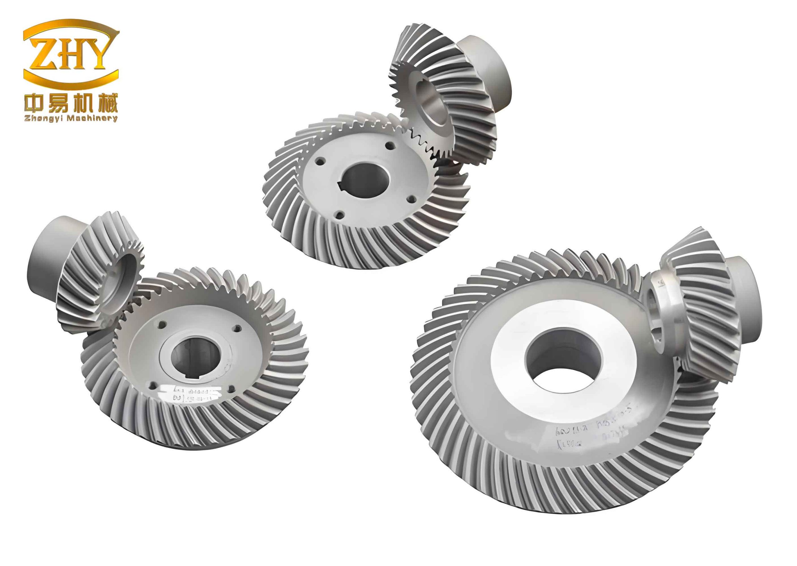
The resulting 3D geometric model, as visualized, is not merely a pictorial representation. It is a mathematically precise digital twin derived from the fundamental manufacturing kinematics. This model serves as the essential input for subsequent advanced engineering analyses.
5. Conclusion and Significance
This exposition has detailed the comprehensive procedure for geometrically modeling Klingelnberg cyclo-palloid hyperboloidal gears. The process begins with a thorough understanding of the continuous generating manufacturing principle, where an extended epicycloidal surface is formed on an imaginary crown gear. By meticulously establishing the kinematic chain of coordinate transformations—linking the rotating cutter blade, the orbiting cutter head on the stationary crown gear, and the rolling workpiece—a general mathematical framework for the tooth flank is developed. The core of this framework is the system combining the locus equation and the meshing condition derived from spatial gearing theory.
To transition from theory to a tangible digital model, a strategy for discretizing the tooth surface and solving the resulting nonlinear equations numerically is implemented. Utilizing computational software like MATLAB enables the efficient calculation of thousands of precise points defining the tooth flank. These points form the bedrock for constructing a smooth, accurate 3D solid model in a CAD environment such as Pro/ENGINEER.
The successfully constructed 3D model of the hyperboloidal gear pair is a critical enabler for modern engineering research and development. It provides the essential geometry for:
- Tooth Contact Analysis (TCA): Simulating the transmission error and contact pattern under load, which is vital for predicting noise, vibration, and durability.
- Manufacturing Simulation and Error Compensation: Comparing the manufactured gear surface (from CMM data) against the theoretical model to identify errors and optimize machine settings.
- Finite Element Analysis (FEA): Performing detailed stress, strain, and root bending fatigue analysis under operational loads.
- Dynamic System Simulation: Integrating the precise gear geometry into multi-body dynamics models to study system-level performance.
Thus, mastering the geometric modeling of complex gear systems like the Klingelnberg cyclo-palloid hyperboloidal gears lays a indispensable foundation for their design optimization, precision manufacturing, and performance validation in demanding applications.