
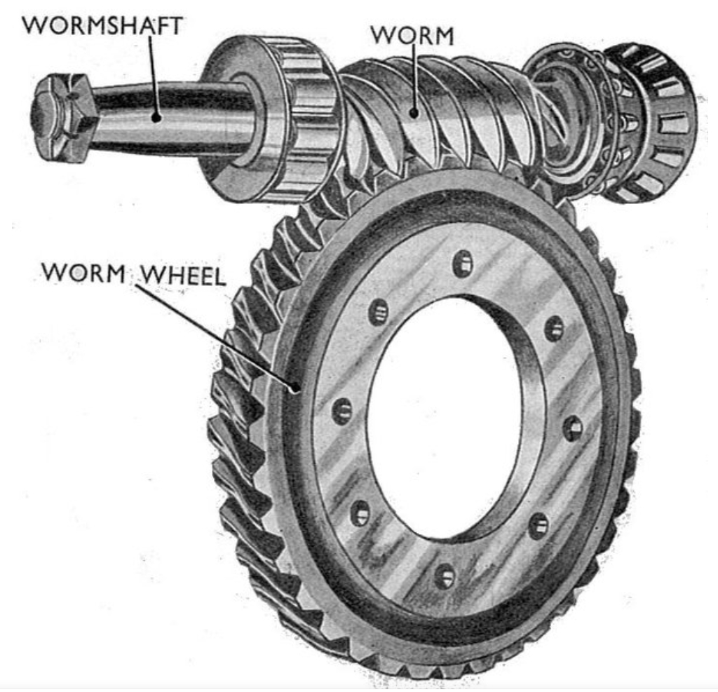
In engineering applications, the worm gear drive is a crucial mechanism for transmitting motion and power between non-intersecting shafts, typically at a 90-degree angle. Its advantages include high transmission ratio, compact structure, smooth operation, and low noise, making it widely used in industries such as mining, metallurgy, transportation, and lifting machinery. However, traditional design methods for worm gear drives often rely on empirical rules and iterative trials, which can be time-consuming and may not yield optimal results. To address the shortcomings of high cost and low efficiency in ordinary cylindrical worm gear drives, I propose a multi-objective fuzzy optimization approach based on Matlab. This method integrates fuzzy set theory to handle uncertainties in design constraints, aiming to minimize the volume of the worm wheel rim and maximize transmission efficiency simultaneously. By establishing a mathematical model, defining membership functions, and utilizing Matlab’s optimization toolbox, I demonstrate a systematic design process that significantly improves performance. This article delves into the detailed formulation, implementation, and results, providing a comprehensive reference for engineers and designers.
The foundation of this optimization lies in constructing a fuzzy optimization mathematical model. In fuzzy optimization, design constraints are treated as fuzzy sets to account for real-world uncertainties, such as variations in material properties or operating conditions. For the worm gear drive, I focus on two primary objectives: reducing the material cost by minimizing the volume of the worm wheel rim and enhancing energy efficiency by maximizing the transmission efficiency. These objectives often conflict, as a smaller volume might compromise strength, while higher efficiency may require larger dimensions. Thus, a multi-objective approach is essential, and fuzzy logic helps balance these trade-offs effectively. The entire process involves selecting design variables, formulating objective functions, defining constraints, and applying fuzzy transformations, all implemented through Matlab programming. This methodology not only streamlines the design but also ensures robustness in practical applications.
Establishment of the Fuzzy Optimization Mathematical Model
The first step in optimizing the worm gear drive is to identify the design variables that significantly influence the objectives. After analyzing the worm gear drive mechanics, I select three independent parameters: the number of worm threads \(z_1\), the module \(m\), and the diameter factor \(q\). These variables control the geometric and performance characteristics of the worm gear drive. Thus, the design vector is defined as:
$$ X = [x_1, x_2, x_3]^T = [z_1, m, q]^T $$
where \(x_1\) represents the worm thread count, \(x_2\) the module, and \(x_3\) the diameter factor. These variables are chosen because they directly affect the size, strength, and efficiency of the worm gear drive, allowing for targeted optimization.
Formulation of Objective Functions
To achieve an optimal worm gear drive design, I establish two objective functions. The first aims to minimize the volume of the worm wheel rim, which is typically made of expensive bronze material, thereby reducing cost. The second objective seeks to maximize the transmission efficiency, which is often low in worm gear drives due to sliding friction. By optimizing both, I aim for a cost-effective and energy-efficient worm gear drive system.
Objective Function 1: Minimization of Worm Wheel Rim Volume
The volume of the worm wheel rim is calculated based on its annular geometry. The outer diameter \(d_e\), inner diameter \(d_0\), and width \(B\) are derived from the worm gear drive parameters. For a worm gear drive with a transmission ratio \(i = 20\) (where \(i = z_2 / z_1\), and \(z_2\) is the number of worm gear teeth), the expressions are:
$$ d_e = m(i z_1 + 3) = m(20 z_1 + 3) $$
$$ d_0 = m(i z_1 – 6.4) = m(20 z_1 – 6.4) $$
$$ B = 0.67 d_{a1} = 0.67 m(q + 2) $$
where \(d_{a1}\) is the tip diameter of the worm. The volume \(V\) is given by:
$$ V = \frac{\pi}{4} (d_e^2 – d_0^2) B $$
Substituting the above equations, the objective function for volume minimization becomes:
$$ f_1(X) = \frac{\pi}{4} \left[ (m(20 z_1 + 3))^2 – (m(20 z_1 – 6.4))^2 \right] \cdot 0.67 m(q + 2) $$
Simplifying this expression, I obtain:
$$ f_1(X) = 0.5262 m^3 (q + 2) \left[ (20 z_1 + 3)^2 – (20 z_1 – 6.4)^2 \right] $$
In terms of design variables, where \(x_1 = z_1\), \(x_2 = m\), and \(x_3 = q\):
$$ f_1(X) = 0.5262 x_2^3 (x_3 + 2) \left[ (20 x_1 + 3)^2 – (20 x_1 – 6.4)^2 \right] $$
This function represents the volume in cubic millimeters, and minimizing it reduces material usage in the worm gear drive.
Objective Function 2: Maximization of Transmission Efficiency
The transmission efficiency \(\eta\) of a worm gear drive is a critical performance metric, typically ranging from 0.75 to 0.92 due to high sliding friction. To incorporate efficiency into the optimization, I maximize \(\eta\), which is equivalent to minimizing its reciprocal. The efficiency formula for a worm gear drive is:
$$ \eta = 0.96 \frac{\tan \lambda}{\tan(\lambda + \rho_v)} $$
where \(\lambda\) is the lead angle of the worm, given by \(\tan \lambda = z_1 / q = x_1 / x_3\), and \(\rho_v\) is the equivalent friction angle, with \(\tan \rho_v = f_v\). The equivalent friction coefficient \(f_v\) depends on the sliding velocity \(v_s\). Based on empirical data from handbooks, I derive a curve-fitting formula for \(f_v\) using Matlab:
$$ f_v = 0.0175192 e^{1.0460682 / v_s} $$
The sliding velocity \(v_s\) is calculated as:
$$ v_s = \frac{m n_1}{19100} \sqrt{z_1^2 + q^2} $$
where \(n_1 = 960\) rpm is the worm speed. Substituting the design variables:
$$ v_s = \frac{x_2 \cdot 960}{19100} \sqrt{x_1^2 + x_3^2} = 0.05026178 x_2 \sqrt{x_1^2 + x_3^2} $$
Thus, the objective function for efficiency maximization, expressed as the minimization of its reciprocal, is:
$$ f_2(X) = \frac{1}{\eta} = \frac{\tan(\lambda + \rho_v)}{0.96 \tan \lambda} $$
Using trigonometric identities and substituting \(\tan \lambda = x_1 / x_3\) and \(\tan \rho_v = f_v\), this simplifies to:
$$ f_2(X) = \frac{x_1 x_3 + f_v x_3^2}{0.96 x_1 x_3 – 0.96 x_1^2 f_v} $$
Here, \(f_v\) is a function of \(v_s\), which in turn depends on \(x_1\), \(x_2\), and \(x_3\). This complexity highlights the nonlinear nature of the worm gear drive efficiency optimization.
Unified Objective Function
To solve the multi-objective optimization problem, I combine the two objective functions into a single unified function using the weighted sum method. This approach assigns weights to each objective based on their relative importance. For the worm gear drive design, I prioritize volume reduction over efficiency improvement, so I set weight \(\omega_1 = 0.8\) for \(f_1(X)\) and \(\omega_2 = 0.2\) for \(f_2(X)\). However, the two functions have different magnitudes: \(f_1(X)\) is on the order of \(10^6\) mm³, while \(f_2(X)\) is dimensionless. To ensure balanced contribution, I scale \(f_2(X)\) by \(10^6\). The unified objective function becomes:
$$ f(X) = \omega_1 f_1(X) + \omega_2 \cdot 10^6 f_2(X) $$
Substituting the values:
$$ f(X) = 0.8 \cdot 0.5262 x_2^3 (x_3 + 2) \left[ (20 x_1 + 3)^2 – (20 x_1 – 6.4)^2 \right] + 0.2 \cdot 10^6 \cdot \frac{x_1 x_3 + f_v x_3^2}{0.96 x_1 x_3 – 0.96 x_1^2 f_v} $$
Simplifying further:
$$ f(X) = 0.420976 x_2^3 (x_3 + 2) \left[ (20 x_1 + 3)^2 – (20 x_1 – 6.4)^2 \right] – \frac{4.8 \times 10^6 (x_1 x_3 + f_v x_3^2)}{x_1 (x_3 – x_1 f_v)} $$
This unified function serves as the primary target for minimization in the worm gear drive optimization, balancing both volume and efficiency considerations.
Construction of Constraint Conditions
In engineering design, constraints ensure that the worm gear drive meets functional and safety requirements. These constraints often have fuzzy boundaries due to uncertainties in material properties, manufacturing tolerances, and operating conditions. I categorize constraints into boundary constraints (geometric limits) and performance constraints (strength and operational limits). For the worm gear drive, I define the following constraints, each expressed as an inequality \(g_j(X) \leq 0\) or with fuzzy allowable ranges.
Boundary Constraints
Boundary constraints define the feasible ranges for design variables based on worm gear drive standards and practical considerations. These include limits on worm thread count, gear teeth, module, and diameter factor. The fuzzy nature arises from permissible deviations in these parameters. I summarize the boundary constraints in Table 1, including both crisp and fuzzy bounds.
| Parameter | Symbol | Standard Range | Fuzzy Lower Bound | Fuzzy Upper Bound | Constraint Expression |
|---|---|---|---|---|---|
| Worm Thread Count | \(z_1\) | 2 to 6 | 1.7 to 2 | 6 to 6.3 | \(2 \leq x_1 \leq 6\) |
| Worm Gear Teeth Count | \(z_2\) | 30 to 80 | 25.5 to 30 | 80 to 84 | \(30 \leq 20 x_1 \leq 80\) |
| Module | \(m\) | 2 to 18 mm | 1.7 to 2 | 18 to 18.9 | \(2 \leq x_2 \leq 18\) |
| Diameter Factor | \(q\) | 8 to 15 | 6.8 to 8 | 15 to 15.75 | \(8 \leq x_3 \leq 15\) |
These constraints ensure that the worm gear drive design adheres to typical specifications while allowing for flexibility through fuzzy intervals.
Performance Constraints
Performance constraints guarantee that the worm gear drive operates reliably under load. These include contact stress, bending stress, shaft deflection, sliding velocity, and thermal balance limits. Each constraint is derived from worm gear drive design formulas and incorporates safety factors. Due to uncertainties in material properties and operating conditions, these constraints are treated as fuzzy. The performance constraints are summarized in Table 2, with detailed formulations below.
| Constraint Type | Symbol | Standard Limit | Fuzzy Lower Bound | Fuzzy Upper Bound | Constraint Expression |
|---|---|---|---|---|---|
| Contact Stress | \(\sigma_H\) | \([\sigma_H] = 166.57\) MPa | 166.57 to 169.92 MPa | 169.92 to 174.9 MPa | \(g_5(X) \leq [\sigma_H]\) |
| Bending Stress | \(\sigma_F\) | \([\sigma_F] = 38.164\) MPa | 38.164 to 38.924 MPa | 38.924 to 40.07 MPa | \(g_6(X) \leq [\sigma_F]\) |
| Shaft Deflection | \(f\) | \([f] = m/50\) mm | \(0.02m\) to \(0.0204m\) mm | \(0.0204m\) to \(0.021m\) mm | \(g_7(X) \leq [f]\) |
| Sliding Velocity | \(v_s\) | \([v_s] = 16\) m/s | 16 to 16.32 m/s | 16.32 to 16.8 m/s | \(g_8(X) \leq [v_s]\) |
| Temperature Rise | \(\Delta t\) | \([\Delta t] = 60^\circ C\) | 60 to 61.2°C | 61.2 to 63°C | \(g_9(X) \leq [\Delta t]\) |
The mathematical expressions for each performance constraint are derived as follows:
1. Contact Stress Constraint: The contact stress \(\sigma_H\) for a worm gear drive is calculated using:
$$ \sigma_H = Z_E \sqrt{\frac{9400 T_2 K_A K_V K_\beta}{d_1 d_2^2}} \leq [\sigma_H] $$
where \(Z_E = 155 \sqrt{\text{MPa}}\) for steel worm and bronze gear, \(T_2 = 1268.36\) N·m is the output torque, \(K_A = 1.0\), \(K_V = 1.1\), \(K_\beta = 1.0\), \(d_1 = m q = x_2 x_3\), and \(d_2 = m i z_1 = 20 x_1 x_2\). Substituting and simplifying:
$$ g_5(X) = \frac{28066.176}{\sqrt{x_1^2 x_2^3 x_3}} \leq [\sigma_H] $$
2. Bending Stress Constraint: The bending stress \(\sigma_F\) is given by:
$$ \sigma_F = \frac{666 T_2 K_A K_V K_\beta}{d_1 d_2 m} Y_{Fs} Y_\beta \leq [\sigma_F] $$
where \(Y_{Fs}\) is the composite tooth form factor, approximated as \(Y_{Fs} = 2.58 e^{-0.049 x_1}\) via curve fitting, and \(Y_\beta = 1 – \lambda/120^\circ\) with \(\lambda = \arctan(x_1/x_3)\). Thus:
$$ g_6(X) = \frac{119866.869 e^{-0.049 x_1} \left(1 – \frac{\arctan(x_1/x_3)}{120}\right)}{x_1 x_2^3 x_3} \leq [\sigma_F] $$
3. Shaft Deflection Constraint: The deflection \(f\) at the worm due to radial and tangential forces must be limited:
$$ f = \frac{\sqrt{F_{r1}^2 + F_{t1}^2}}{48 E I} L^3 \leq [f] $$
with \(F_{t1} = 2T_2 / (i \eta m q)\), \(F_{r1} = 2T_2 \tan \alpha / (m i z_1)\), \(\alpha = 20^\circ\), \(E = 2.1 \times 10^5\) MPa, \(I = \pi m^4 (q – 2.4)^4 / 64\), \(L = 1.1 m (i z_1 + 2) = 1.1 x_2 (20 x_1 + 2)\), and \([f] = m/50\). After simplification:
$$ g_7(X) = \frac{3.411852 \times 10^{-4} (20 x_1 + 2)^3 \sqrt{(0.36397/x_1)^2 + (1.17647/x_3)^2}}{(x_3 – 2.4)^4 x_2^2} \leq 0.0204 x_2 $$
4. Sliding Velocity Constraint: To prevent excessive wear and overheating:
$$ v_s = \frac{m n_1}{19100} \sqrt{z_1^2 + q^2} \leq [v_s] $$
leading to:
$$ g_8(X) = 0.05026178 x_2 \sqrt{x_1^2 + x_3^2} \leq [v_s] $$
5. Thermal Balance Constraint: For closed worm gear drives, the temperature rise \(\Delta t\) must be controlled:
$$ \Delta t = \frac{1000 P (1 – \eta)}{k_s A} \leq [\Delta t] $$
where \(P = 7.5\) kW is input power, \(\eta = 0.85\) assumed, \(k_s = 15\) W/(m²·°C), and \(A = 0.33 (a/100)^{1.75}\) with \(a = (d_1 + d_2)/2 = m(q + i z_1)/2 = x_2(x_3 + 20 x_1)/2\). Thus:
$$ g_9(X) = \frac{2417407.226}{[x_2 (x_3 + 20 x_1)]^{1.75}} \leq [\Delta t] $$
These constraints ensure the worm gear drive’s structural integrity and operational efficiency under typical loading conditions.
Fuzzy Constraint Membership Functions and Non-Fuzzy Processing
In fuzzy optimization, constraints are represented by membership functions that quantify the degree of satisfaction. For the worm gear drive design, I use linear membership functions due to their simplicity and effectiveness in engineering applications. The membership function \(\mu_{g_j}(X)\) for a performance constraint \(g_j(X)\) defines how well a design point meets the constraint, ranging from 0 (完全不允许) to 1 (完全允许). Similarly, for boundary constraints, membership functions handle the fuzzy boundaries of design variables.
Membership Function Definitions
For performance constraints, the linear membership function is expressed as:
$$ \mu_{g_j}(X) =
\begin{cases}
1 & \text{if } g_j(X) \leq \sigma_j^l \\
\frac{\sigma_j^u – g_j(X)}{\sigma_j^u – \sigma_j^l} & \text{if } \sigma_j^l \leq g_j(X) \leq \sigma_j^u \\
0 & \text{if } g_j(X) \geq \sigma_j^u
\end{cases} $$
where \(\sigma_j^l\) and \(\sigma_j^u\) are the lower and upper bounds of the fuzzy allowable interval for constraint \(j\). These bounds represent the transition from fully allowable to fully unallowable states. For boundary constraints on design variables, the membership function for a variable \(x_j\) is defined as:
$$ \mu_{x_j} =
\begin{cases}
0 & \text{if } x_j \leq \underline{x}_j^l \\
\frac{x_j – \underline{x}_j^l}{\underline{x}_j^u – \underline{x}_j^l} & \text{if } \underline{x}_j^l \leq x_j \leq \underline{x}_j^u \\
1 & \text{if } \underline{x}_j^u \leq x_j \leq \overline{x}_j^l \\
\frac{\overline{x}_j^u – x_j}{\overline{x}_j^u – \overline{x}_j^l} & \text{if } \overline{x}_j^l \leq x_j \leq \overline{x}_j^u \\
0 & \text{if } x_j \geq \overline{x}_j^u
\end{cases} $$
where \(\underline{x}_j^l\) and \(\underline{x}_j^u\) are the lower bounds of the fuzzy interval, and \(\overline{x}_j^l\) and \(\overline{x}_j^u\) are the upper bounds. This formulation allows for smooth transitions at both ends of the allowable range, accommodating uncertainties in the worm gear drive parameters.
Determination of Fuzzy Allowable Intervals
The fuzzy allowable intervals are established using the expansion coefficient method, which incorporates engineering experience and design standards. For performance constraints, I define expansion coefficients \(\beta^l = 0.85\) for the lower bound and \(\beta^u = 1.05\) for the upper bound, applied to the standard allowable values. For boundary constraints, similar coefficients are used based on typical tolerances. The resulting fuzzy intervals are summarized in Tables 1 and 2 earlier. For example, the contact stress allowable \([\sigma_H] = 166.57\) MPa has a fuzzy lower bound from 166.57 to 169.92 MPa and a fuzzy upper bound from 169.92 to 174.9 MPa. These intervals reflect the inherent vagueness in material properties and operating conditions for worm gear drives.
Optimal Level Cut Set Determination
To convert the fuzzy optimization problem into a crisp one, I determine the optimal level cut set \(\lambda^*\) using fuzzy comprehensive evaluation. This involves assessing factors like design safety, cost, and manufacturability. Through weighted evaluation of these factors, I compute \(\lambda^* = 0.6\), indicating that designs with membership degrees above 0.6 are considered acceptable. This value balances conservatism and optimality in the worm gear drive design.
Non-Fuzzy Processing
Using \(\lambda^* = 0.6\), I transform the fuzzy constraints into crisp equivalents by applying the level cut operation. For a membership function \(\mu_{g_j}(X) \geq \lambda^*\), the constraint becomes \(g_j(X) \leq \sigma_j^u – \lambda^* (\sigma_j^u – \sigma_j^l)\). Similarly, for boundary constraints, the feasible ranges are adjusted. The resulting non-fuzzy optimization model for the worm gear drive is:
Minimize \(f(X)\) subject to:
$$ 1.88 \leq x_1 \leq 6.12 $$
$$ 28.2 \leq 20 x_1 \leq 81.6 $$
$$ 1.88 \leq x_2 \leq 18.36 $$
$$ 7.52 \leq x_3 \leq 15.35 $$
$$ g_5(X) \leq 169.92 $$
$$ g_6(X) \leq 38.924 $$
$$ g_7(X) \leq 0.0204 x_2 $$
$$ g_8(X) \leq 16.32 $$
$$ g_9(X) \leq 61.2 $$
This crisp model can be solved using conventional optimization techniques, facilitating the implementation in Matlab.
Matlab Programming and Optimization Solution
To solve the non-fuzzy optimization problem, I utilize Matlab’s Optimization Toolbox, specifically the fmincon function for constrained nonlinear optimization. The process involves writing M-files for the objective function and constraints, setting up variable bounds, and executing the optimization. This approach leverages Matlab’s computational power to efficiently find the optimal worm gear drive parameters.
Objective Function M-File
I create a file named myobj.m that defines the unified objective function \(f(X)\). The code includes the expressions for \(f_1(X)\) and \(f_2(X)\), with \(f_v\) computed based on \(v_s\). The Matlab code is as follows:
function f = myobj(x)
% x(1) = z1, x(2) = m, x(3) = q
vs = 0.05026178 * x(2) * sqrt(x(1)^2 + x(3)^2);
fv = 0.0175192 * exp(1.0460682 / vs);
f1 = 0.420976 * x(2)^3 * (x(3) + 2) * ((20*x(1) + 3)^2 - (20*x(1) - 6.4)^2);
f2 = (4.8e6 * (x(1)*x(3) + fv*x(3)^2)) / (x(1) * (x(3) - x(1)*fv));
f = f1 - f2; % Note: f2 is subtracted due to sign in unified function
end
This function computes the value of \(f(X)\) for any given design vector \(X\), enabling the optimizer to minimize it.
Nonlinear Constraint M-File
The constraints are implemented in a file named mycon.m, which returns the inequality constraints \(c(X) \leq 0\) and equality constraints \(ceq(X) = 0\). For the worm gear drive, all constraints are inequalities. The code is:
function [c, ceq] = mycon(x)
vs = 0.05026178 * x(2) * sqrt(x(1)^2 + x(3)^2);
fv = 0.0175192 * exp(1.0460682 / vs);
% Contact stress constraint
c1 = 28066.176 / sqrt(x(1)^2 * x(2)^3 * x(3)) - 169.92;
% Bending stress constraint
c2 = 119866.869 * exp(-0.049*x(1)) * (1 - atan(x(1)/x(3))/120) / (x(1)*x(2)^3*x(3)) - 38.924;
% Shaft deflection constraint
c3 = 3.411852e-4 * (20*x(1) + 2)^3 * sqrt((0.36397/x(1))^2 + (1.17647/x(3))^2) / ((x(3)-2.4)^4 * x(2)^2) - 0.0204*x(2);
% Sliding velocity constraint
c4 = 0.05026178 * x(2) * sqrt(x(1)^2 + x(3)^2) - 16.32;
% Thermal balance constraint
c5 = 2417407.226 / (x(2) * (x(3) + 20*x(1)))^1.75 - 61.2;
c = [c1; c2; c3; c4; c5];
ceq = [];
end
These constraints ensure that the optimized worm gear drive meets all performance requirements.
Optimization Setup and Execution
In the main script, I define the variable bounds, linear constraints, initial guess, and optimization options. The bounds correspond to the non-fuzzy ranges from the level cut set. The code is:
lb = [1.7; 1.7; 6.8]; % Lower bounds
ub = [6.3; 18.9; 15.75]; % Upper bounds
x0 = [1.7; 1.7; 6.8]; % Initial guess
A = [-1 0 0; 1 0 0; 0 -1 0; 0 1 0; 0 0 -1; 0 0 1]; % Linear inequalities for bounds
b = [-1.88; 6.12; -1.88; 18.36; -7.52; 15.35]; % Corresponding values
options = optimset('Display', 'off', 'LargeScale', 'off');
[x_opt, fval] = fmincon(@myobj, x0, A, b, [], [], lb, ub, @mycon, options);
Running this script yields the optimal design variables for the worm gear drive. The result is \(x_1 = 4.08\), \(x_2 = 4.743\), \(x_3 = 15.35\). After rounding to standard values for practicality, the final worm gear drive parameters are: worm thread count \(z_1 = 4\), module \(m = 5\) mm, and diameter factor \(q = 15\).
Optimization Results and Discussion
To evaluate the improvement, I compare the optimized design with a traditional design using typical parameters: \(z_1 = 2\), \(m = 8\) mm, \(q = 10\). For the traditional worm gear drive, the worm wheel rim volume \(V\) and transmission efficiency \(\eta\) are computed as:
$$ V = 0.5262 \times 8^3 \times (10 + 2) \times [(20 \times 2 + 3)^2 – (20 \times 2 – 6.4)^2] = 2.327958 \times 10^6 \text{ mm}^3 $$
$$ \eta = 0.96 \frac{\tan(\arctan(2/10))}{\tan(\arctan(2/10) + \rho_v)} \approx 0.8586 \text{ (with } f_v \text{ computed)} $$
For the optimized worm gear drive with \(z_1 = 4\), \(m = 5\) mm, \(q = 15\):
$$ V^* = 0.5262 \times 5^3 \times (15 + 2) \times [(20 \times 4 + 3)^2 – (20 \times 4 – 6.4)^2] = 1.64606 \times 10^6 \text{ mm}^3 $$
$$ \eta^* = 0.96 \frac{\tan(\arctan(4/15))}{\tan(\arctan(4/15) + \rho_v)} \approx 0.8787 $$
The percentage improvements are:
Volume reduction: \(\frac{2.327958 – 1.64606}{2.327958} \times 100\% = 29.3\%\)
Efficiency increase: \(\frac{0.8787 – 0.8586}{0.8586} \times 100\% = 2.34\%\)
These results demonstrate that the fuzzy optimization approach successfully reduces material cost and enhances energy efficiency for the worm gear drive. The volume reduction is significant, leading to cost savings, while the efficiency improvement, though modest, contributes to better performance over the worm gear drive’s lifespan.
Conclusion
In this article, I have presented a comprehensive multi-objective fuzzy optimization design method for cylindrical worm gear drives based on Matlab. By integrating fuzzy set theory, I addressed uncertainties in design constraints, aiming to minimize worm wheel rim volume and maximize transmission efficiency. The mathematical model incorporated key design variables, objective functions, and fuzzy constraints, with non-fuzzy processing via an optimal level cut set. Implementation in Matlab using the Optimization Toolbox yielded an optimized worm gear drive design with substantial volume reduction and improved efficiency compared to traditional methods. This approach not only streamlines the design process but also provides a robust framework for handling real-world variabilities. The methodology is applicable to various worm gear drive applications, offering valuable insights for engineers seeking cost-effective and efficient solutions. Future work could explore additional objectives, such as weight minimization or noise reduction, and extend the fuzzy logic to dynamic operating conditions for enhanced worm gear drive performance.