
Gears are critical components in mechanical equipment, with CNC gear hobbing being a predominant manufacturing method for cylindrical, bevel, and worm gears. This process enhances efficiency, precision, and product quality, yet optimizing its numerous coupled parameters remains challenging. This study addresses CNC gear hobbing parameter optimization through a multi-objective framework, minimizing energy consumption, time, and quality error.
Problem Formulation for Gear Hobbing Optimization
The multi-objective optimization problem comprises decision variables, constraints, and objectives:
Decision Variables
Key optimizable parameters in gear hobbing include:
- Number of hob heads \(z_0\)
- Hob outer diameter \(d_{a0}\) (mm)
- Spindle speed \(n_0\) (r/min)
- Axial feed rate \(f\) (mm/rev)
Workpiece parameters (module \(m\), teeth count \(z_1\), pressure angle \(\alpha\), etc.) are treated as fixed inputs.
Constraints
Optimization is bounded by practical and physical limits:
| Constraint Type | Mathematical Expression |
|---|---|
| Boundary | \(z_{0,\text{min}} \leq z_0 \leq z_{0,\text{max}}\) \(d_{a0,\text{min}} \leq d_{a0} \leq d_{a0,\text{max}}\) \(n_{0,\text{min}} \leq n_0 \leq n_{0,\text{max}}\) \(f_{\text{min}} \leq f \leq f_{\text{max}}\) |
| Precision | \(z_0, n_0 \in \mathbb{Z}\); \(d_{a0}, f\) discretized to 2 decimals |
| Tool Availability | \((z_0, d_{a0}) \in H\), where \(H\) is the hob repository |
| Cutting Force | \(F_c \leq F_{c,\text{max}}\) |
| Surface Roughness | \(\frac{f^2}{r_t} \leq 0.0312 \cdot \text{Ra}\), \(r_t\) = tool tip radius |
Objective Functions
Three objectives are minimized:
- Energy Consumption \(E\) (kWh):
$$E = \frac{E_s + E_a + E_c}{60000}$$
where \(E_s\), \(E_a\), \(E_c\) represent standby, air-cutting, and cutting energy. - Time \(T\) (s):
$$T = (T_s + T_a + T_c) \times 60$$
comprising standby, air-cutting, and cutting durations. - Quality Error \(Q\) (mm):
$$Q = \omega_1 \delta_1 + \omega_2 \delta_2$$
with \(\delta_1 = \frac{4f}{\pi z_0} \sin \alpha\) (profile error) and \(\delta_2 = \frac{4f}{m z_1} \sin \alpha\) (helical error).
The multi-objective problem is formalized as:
$$\min_{\mathbf{e}} \left( E(\mathbf{e}), T(\mathbf{e}), Q(\mathbf{e}) \right)$$
where \(\mathbf{e} = (z_0, d_{a0}, n_0, f)\).
HDBSCAN-Based Parameter Range Identification
Historical gear hobbing cases \(\mathcal{C}_h\) are clustered to identify feasible parameter ranges for new workpieces. HDBSCAN (Hierarchical Density-Based Spatial Clustering) processes cases as follows:
- Data Transformation: Normalize parameters to [0,1] range.
- Minimum Spanning Tree (MST): Construct MST using mutual reachability distances.
- Hierarchical Tree: Build cluster hierarchy by removing MST edges in descending weight order.
- Tree Condensation: Simplify hierarchy using minimum cluster size (\(mcs = 3\)).
- Cluster Extraction: Select the most relevant cluster for the target workpiece.
Parameter bounds \(\mathbf{ul}\), \(\mathbf{ll}\) are derived from the selected cluster’s extrema, expanded by 5% for robustness:
$$\mathbf{ul} = \left( z_{0,\text{max}}, d_{a0,\text{max}}, n_{0,\text{max}}, f_{\text{max}} \right)$$
$$\mathbf{ll} = \left( z_{0,\text{min}}, d_{a0,\text{min}}, n_{0,\text{min}}, f_{\text{min}} \right)$$
This ensures feasible initial ranges for optimization.
GMOMPA for Multi-objective Optimization
Guided Multi-Objective Marine Predators Algorithm (GMOMPA) evolves a population \(\text{Prey}\) (100 solutions) over 300 iterations. Elite solutions \(\text{Predator}\) guide the search using three velocity-based phases:
Phase 1: High-Velocity Ratio (Iter < max_iter/3)
Exploration dominates; all solutions perform Brownian motion:
$$\text{step}_i = \mathbf{R}_B \otimes (\text{Predator}_i – \text{Prey}_i)$$
$$\text{Prey}_i = \text{Prey}_i + P \cdot \mathbf{R} \otimes \text{step}_i$$
where \(\mathbf{R}_B\) = Brownian vector, \(\mathbf{R} \sim U(0,1)\), \(P = 0.5\), \(\otimes\) = Hadamard product.
Phase 2: Unit-Velocity Ratio (max_iter/3 ≤ Iter ≤ 2×max_iter/3)
Balanced exploration-exploitation. Top 50% solutions use Lévy motion:
$$\text{step}_i = \mathbf{R}_L \otimes (\text{Predator}_i – \text{Prey}_i)$$
$$\text{Prey}_i = \text{Prey}_i + P \cdot \mathbf{R} \otimes \text{step}_i$$
Bottom 50% follow elite-guided Brownian motion:
$$\text{step}_i = \mathbf{R}_B \otimes (\text{Predator}_i – \text{Prey}_i)$$
$$\text{Prey}_i = \text{Prey}_i + \text{CF} \cdot \mathbf{R} \otimes \text{step}_i$$
with adaptive parameter \(\text{CF} = \left(1 – \frac{\text{iter}}{\text{max\_iter}}\right)^{2}\).
Phase 3: Low-Velocity Ratio (Iter > 2×max_iter/3)
Exploitation intensifies; all solutions adopt Lévy motion:
$$\text{step}_i = \mathbf{R}_L \otimes (\text{Predator}_i – \text{Prey}_i)$$
$$\text{Prey}_i = \text{Prey}_i + \text{CF} \cdot P \cdot \mathbf{R} \otimes \text{step}_i$$
$$\mathbf{R}_L = \text{Lévy vector}, \quad \mathbf{R}_L \sim \frac{0.05 \times u}{|v|^{1/1.5}}$$
FADs Effect
Avoid local optima via Fish Aggregating Devices (probability = 0.2):
$$\text{Prey}_i = \begin{cases}
\text{Prey}_i + \text{CF} \left[ \mathbf{ll} + \mathbf{R} \otimes (\mathbf{ul} – \mathbf{ll}) \right] \otimes \mathbf{U}} & \text{if } r \leq \text{FADs} \\
\text{Prey}_i + \left[ \text{FADs}(1 – r) + r \right] (\text{Prey}_{r1} – \text{Prey}_{r2}) & \text{else}
\end{cases}$$
where \(\mathbf{U}\) = binary vector, \(r, r_1, r_2\) = randoms.
Improved TOPSIS for Solution Ranking
GMOMPA’s Pareto archive (99 solutions) is ranked using AHP-weighted TOPSIS:
- AHP Weighting: Assign weights \(\mathbf{w} = (w_E, w_T, w_Q)\) based on pairwise objective importance (e.g., \(E\):\(T\)=2:1, \(E\):\(Q\)=3:1).
- Distance-Weighted TOPSIS:
- Normalize objective matrix \(\mathbf{X}\) to \(\mathbf{R}\).
- Compute weighted matrix \(\mathbf{V} = \mathbf{R} \times \text{diag}(\mathbf{w})\).
- Identify ideal (\(A^+\)) and anti-ideal (\(A^-\)) solutions:
$$A^+ = (\min V_{E}, \min V_{T}, \min V_{Q}), \quad A^- = (\max V_{E}, \max V_{T}, \max V_{Q})$$ - Calculate Euclidean distances:
$$d_i^+ = \sqrt{\sum_{j} (V_{ij} – A_j^+)^2}, \quad d_i^- = \sqrt{\sum_{j} (V_{ij} – A_j^-)^2}$$ - Rank by relative closeness \(\delta_i = \frac{d_i^-}{d_i^+ + d_i^-}\).
Validation and Comparative Analysis
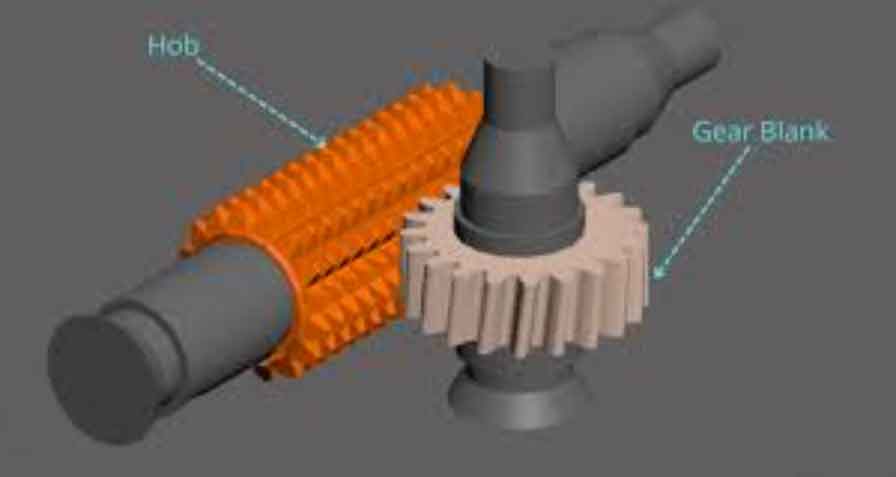
A cylindrical gear (45 steel, \(m = 4\text{mm}\), \(z_1 = 16\), \(\alpha = 20^\circ\)) was processed on a YK3118B-CNC hobbing machine.
Feasibility Validation
HDBSCAN clustered 30 historical gear hobbing cases, identifying key parameters:
$$\mathbf{ul} = (2, 92.52, 1098, 0.80), \quad \mathbf{ll} = (2, 76.48, 922, 0.50)$$
GMOMPA achieved convergence in 300 iterations (Fig. 1), yielding a uniform Pareto front (Fig. 2). Top-ranked solutions balanced objectives effectively (Table 1).
| Rank | \(z_0\) | \(d_{a0}\) (mm) | \(n_0\) (r/min) | \(f\) (mm/rev) | \(E\) (kWh) | \(T\) (s) | \(Q\) (mm) | \(\delta_i\) |
|---|---|---|---|---|---|---|---|---|
| 1 | 2 | 76.50 | 1092 | 0.80 | 0.5741 | 393.69 | 0.00182 | 0.872 |
| 2 | 2 | 78.20 | 1078 | 0.78 | 0.5812 | 398.45 | 0.00179 | 0.843 |
| 3 | 2 | 80.10 | 1055 | 0.75 | 0.5924 | 402.17 | 0.00175 | 0.815 |
| 4 | 2 | 82.30 | 1033 | 0.72 | 0.6038 | 408.92 | 0.00170 | 0.794 |
| 5 | 2 | 85.60 | 1015 | 0.68 | 0.6271 | 415.74 | 0.00163 | 0.763 |
Algorithm Comparison
GMOMPA outperformed MOPSO and NSGA-II in solution diversity and extremum objectives (Fig. 3, Table 2):
| Algorithm | \(\min E\) (kWh) | \(\min T\) (s) | \(\min Q\) (mm) | Hypervolume |
|---|---|---|---|---|
| GMOMPA | 0.5741 | 393.69 | 0.00158 | 0.841 |
| MOPSO | 0.6014 (+4.75%) | 409.15 (+3.93%) | 0.00161 (+1.90%) | 0.792 |
| NSGA-II | 0.5766 (+0.43%) | 395.19 (+0.38%) | 0.00158 (=) | 0.806 |
Conclusion
This study presents an integrated framework for multi-objective optimization in CNC gear hobbing. By combining HDBSCAN clustering for parameter range identification, GMOMPA for efficient Pareto front generation, and improved TOPSIS for decision-making, the method effectively minimizes energy consumption, time, and quality error. Experimental validation confirms superior performance over MOPSO and NSGA-II, with GMOMPA reducing energy by 4.75% and time by 3.93% compared to state-of-the-art methods. Future work will extend this approach to multi-pass gear hobbing and real-time adaptive optimization.