
In the field of precision machinery, the RV reducer stands out as a critical component due to its compact design, high transmission ratio, and reliability. As an essential part of robotic joints and aerospace systems, understanding the dynamic behavior of the RV reducer is paramount for ensuring performance and longevity. In this article, I aim to delve into the theoretical modeling of the RV reducer to analyze its natural frequencies, which are fundamental for resonance response assessment. By establishing a detailed dynamics model and solving the governing equations, I will provide insights into the system’s vibrational characteristics and the influence of material properties on the first-order natural frequency. Throughout this discussion, the term ‘RV reducer’ will be frequently emphasized to highlight its centrality in this analysis.
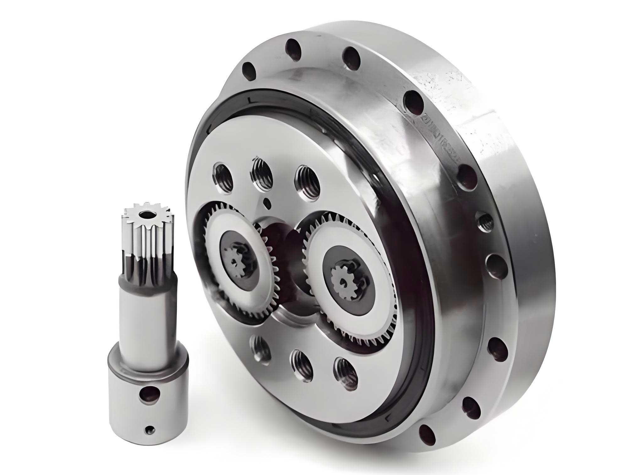
The RV reducer, a two-stage transmission device, combines a planetary gear system with a cycloidal drive mechanism. Its operation begins with the rotation of the sun gear, which drives the planetary gears. These planetary gears are connected to crank shafts via splines, and the crank shafts, in turn, drive cycloid wheels through eccentric motions. The interaction between the cycloid wheels and the fixed pin gear housing results in the rotation of the output carrier. This intricate mechanism allows the RV reducer to achieve high reduction ratios in a compact form. To visualize this structure, consider the following representation:
For dynamic analysis, I adopt a lumped mass approach to model the RV reducer. This method simplifies the system by representing components as point masses connected by springs that account for stiffnesses such as torsional, bearing, and mesh stiffnesses. The model considers 16 degrees of freedom, including tangential motions of the crank shafts and cycloid wheels, to capture the essential dynamics. Key assumptions are made to streamline the analysis: mass centers coincide with geometric centers, stiffnesses are treated as constants, damping and friction are neglected, forces are equivalent to concentrated stresses, and errors are ignored. These assumptions allow for a linear model focused on inherent vibrational properties.
The dynamics of the RV reducer are governed by Newton’s second law and fixed-axis rotation differential equations. For the planetary gear stage, the relative displacements between components lead to elastic forces. For instance, the relative displacement between the sun gear and a planetary gear in the mesh direction is given by:
$$ \phi_{sp} = r_s \theta_s – r_p \theta_{pi} – x_{hi} \cos \alpha $$
where \( r_s \) and \( r_p \) are base circle radii, \( \theta_s \) and \( \theta_{pi} \) are angular displacements, \( x_{hi} \) is the translational displacement of the crank shaft-planetary gear assembly, and \( \alpha \) is the pressure angle. The mesh force is then:
$$ F_{spi} = k_p (r_s \theta_s – r_p \theta_{pi} – x_{hi} \cos \alpha) $$
Here, \( k_p \) denotes the mesh stiffness of the planetary gears. Similarly, for the cycloidal stage, the interaction between the crank shaft and cycloid wheel involves both rotational and translational degrees. The relative displacement in the tangential direction is expressed as:
$$ \phi_{qc} = \theta_{hi} \mp x_{hi} \cos \beta_i \pm \theta_{cj} \cos \beta_i – x_{cj} $$
where \( \beta_i = \beta + (i-1)\frac{2\pi}{3} \), with \( \beta \) being the angle between the crank throw and the x-axis. The force from the bearing is:
$$ F_{hicj} = k_n \phi_{qc} $$
with \( k_n \) as the bearing stiffness. The mesh between the cycloid wheel and pin gear has a relative displacement:
$$ \phi_{ckj} = x_{cj} – \theta_{cj} r_c $$
and the corresponding force is:
$$ F_{ckj} = k_g \phi_{ckj} $$
where \( k_g \) is the cycloid-pin mesh stiffness. The output carrier is driven by the crank shaft’s revolution, with a relative displacement:
$$ \phi_{ohi} = x_{hi} – \theta_o r_h $$
and force:
$$ F_{ohi} = k_m \phi_{ohi} $$
where \( k_m \) is the support bearing stiffness. Based on these interactions, the equations of motion for each component are derived. For example, the sun gear’s dynamics are:
$$ J_s \ddot{\theta}_s = k_b (\theta_a – \theta_s) + \sum_{i=1}^{3} F_{spi} r_s $$
where \( J_s \) is the moment of inertia, \( k_b \) is the input shaft torsional stiffness, and \( \theta_a \) is the input shaft angle. The planetary gear’s rotation is described by:
$$ J_p \ddot{\theta}_{pi} = F_{spi} r_p + k_q (\theta_{hi} – \theta_{pi}) $$
with \( J_p \) as the planetary gear’s inertia and \( k_q \) as the crank shaft torsional stiffness. The crank shaft’s rotation equation is:
$$ J_h \ddot{\theta}_{hi} = k_q (\theta_{pi} – \theta_{hi}) – \sum_{j=1}^{2} (e \cdot F_{hicj}) $$
where \( J_h \) is the crank shaft’s inertia and \( e \) is the eccentricity. The translational motion of the crank shaft-planetary gear assembly is:
$$ (m_p + m_h) \ddot{x}_{hi} = F_{spi} \cos \alpha + \sum_{j=1}^{2} F_{hicj} + k_m (\theta_o r_h – x_{hi}) $$
The cycloid wheel’s equations include rotation:
$$ J_c \ddot{\theta}_{cj} = F_{ckj} r_c – \sum_{i=1}^{3} r_h F_{hicj} $$
and translation:
$$ m_c \ddot{x}_{cj} = \sum_{i=1}^{3} F_{hicj} – F_{ckj} $$
Finally, the output carrier’s dynamics are:
$$ J_o \ddot{\theta}_o = T_c + \sum_{i=1}^{3} r_h F_{ohi} $$
where \( J_o \) is the carrier’s inertia and \( T_c \) is the output torque. These equations collectively form the system’s free vibration dynamics, represented in matrix form as:
$$ [M] \{\ddot{x}\} + [K] \{x\} = 0 $$
Here, \( [M] \) is the mass matrix and \( [K] \) is the stiffness matrix, both of size 16×16. The mass matrix is diagonal, while the stiffness matrix is symmetric, incorporating all stiffness terms from the model.
To solve for the natural frequencies, the parameters in these matrices must be determined. For the RV reducer under study, which is based on the RV-320E model, I calculate masses and moments of inertia using 3D modeling software to ensure accuracy, as components like the cycloid wheel have complex geometries. Stiffnesses are computed based on mechanical principles. For torsional stiffness of shafts, the formula for a cylindrical shaft is:
$$ k = \frac{G \pi d^4}{32 l} $$
where \( G \) is the shear modulus, \( d \) is the diameter, and \( l \) is the length. For stepped shafts, the reciprocal of stiffnesses are summed. Bearing stiffnesses are derived from radial force and deformation relationships, while mesh stiffnesses for gears involve tooth geometry and material properties. Specifically, the planetary gear mesh stiffness \( k_p \) is calculated using:
$$ k_p = c’ (0.75 \varepsilon_a + 0.25) $$
with \( c’ = C_M C_R C_B b / q \), where \( \varepsilon_a \) is the contact ratio. For the cycloid-pin mesh, the equivalent torsional stiffness \( K_{bc} \) is obtained by summing contributions from individual engaged teeth:
$$ K_{bc} = \sum_{i=2}^{13} K_i l_i^2 $$
where \( K_i \) is the contact stiffness for each tooth pair and \( l_i \) is the distance from the mesh point to the cycloid wheel center. The computed parameters are summarized in the following tables to provide a clear overview of the RV reducer’s characteristics.
| Component | Mass (kg) | Moment of Inertia (kg·m²) |
|---|---|---|
| Input Shaft | 0.85 | 0.0021 |
| Sun Gear | 0.92 | 0.0035 |
| Planetary Gear | 0.78 | 0.0028 |
| Crank Shaft | 1.15 | 0.0042 |
| Cycloid Wheel | 2.34 | 0.0087 |
| Output Carrier | 3.56 | 0.0125 |
| Stiffness Type | Symbol | Value |
|---|---|---|
| Input Shaft Torsional Stiffness | \( k_b \) | 9.5077 × 10⁴ N·m/rad |
| Crank Shaft Torsional Stiffness | \( k_q \) | 6.8493 × 10⁴ N·m/rad |
| Planetary Gear Mesh Stiffness | \( k_p \) | 2.235 × 10⁸ N/m |
| Cycloid-Pin Mesh Stiffness | \( k_g \) | 1.7307 × 10⁸ N·m/rad |
| Needle Bearing Stiffness | \( k_n \) | 4.0668 × 10⁸ N/m |
| Support Bearing Stiffness | \( k_m \) | 1.424 × 10⁸ N/m |
With these parameters, the mass and stiffness matrices are constructed. The stiffness matrix \( [K] \) is populated with elements that couple the various degrees of freedom, such as \( k_{00} = k_b \), \( k_{11} = k_b + 3k_p r_s^2 \), and so on, as detailed in the model. Using MATLAB, the eigenvalue problem \( [K] \{x\} = \omega^2 [M] \{x\} \) is solved to obtain the natural frequencies \( \omega \). The results for the first 10 natural frequencies are listed below, demonstrating the vibrational spectrum of the RV reducer.
| Mode Number | Natural Frequency (Hz) |
|---|---|
| 1 | 1042.8 |
| 2 | 2328.1 |
| 3 | 10422.4 |
| 4 | 13067.8 |
| 5 | 15367.3 |
| 6 | 15561.8 |
| 7 | 16733.1 |
| 8 | 20351.6 |
| 9 | 23135.9 |
| 10 | 23491.9 |
Among these frequencies, the first-order natural frequency is particularly critical because lower frequencies are more susceptible to resonance from external excitations. To understand how material properties affect this frequency, I conduct a sensitivity analysis by varying individual stiffnesses and inertias while keeping other parameters constant. This approach isolates the influence of each component on the RV reducer’s dynamics. The results are presented in graphical form through derived data, showing the percent change in the first-order natural frequency relative to changes in stiffness or inertia.
For stiffness variations, I consider a range from 50% to 150% of the nominal values. The support bearing stiffness \( k_m \) has the most pronounced effect, as it directly couples the crank shaft motion to the output carrier. A plot of the impact reveals that increasing \( k_m \) by 50% raises the first-order natural frequency by approximately 15%, whereas decreasing it by 50% lowers the frequency by about 20%. In contrast, changes in other stiffnesses, such as the input shaft torsional stiffness \( k_b \) or the planetary mesh stiffness \( k_p \), result in less than 5% variation. This underscores the importance of the support bearing in the RV reducer’s vibrational behavior.
Similarly, for inertia variations, the output carrier’s moment of inertia \( J_o \) exerts the greatest influence. Increasing \( J_o \) by 50% decreases the first-order natural frequency by roughly 12%, while reducing it by 50% increases the frequency by 10%. Other inertias, like those of the planetary gears or cycloid wheels, cause changes below 3%. These findings highlight that in designing an RV reducer, optimizing the support bearing stiffness and the output carrier’s inertia can effectively tune the system to avoid resonance frequencies, thereby enhancing performance and durability.
To further elucidate these relationships, I derive mathematical expressions for the sensitivity. The first-order natural frequency \( f_1 \) can be approximated from the system’s eigenvalues. For small changes, the sensitivity coefficient \( S \) for a parameter \( p \) is defined as \( S = \frac{\partial f_1}{\partial p} \cdot \frac{p}{f_1} \). From the dynamics equations, it can be shown that for the support bearing stiffness, the sensitivity is high due to its role in the translational coupling of the crank shaft. Specifically, from the equation for \( x_{hi} \), the term \( k_m (\theta_o r_h – x_{hi}) \) introduces a stiffness that affects the overall system frequency. Similarly, the output carrier’s inertia appears in the denominator of frequency terms, as seen in the characteristic equation derived from \( [K] – \omega^2 [M] = 0 \).
In practical terms, this analysis suggests that when developing an RV reducer, engineers should prioritize selecting high-stiffness support bearings and lightweight materials for the output carrier to achieve higher natural frequencies, thus pushing resonance thresholds beyond operational ranges. For instance, in robotic applications where the RV reducer experiences variable loads, a well-tuned first-order natural frequency can mitigate vibrations that impair precision. Additionally, this model can be extended to include damping effects for forced vibration analysis, but as noted, damping primarily affects amplitude rather than natural frequency in linear systems.
The theoretical framework presented here is validated through consistency with prior studies on RV reducer dynamics. The use of a 16-degree-of-freedom model captures essential features like the tangential motions of crank shafts and cycloid wheels, which are often overlooked in simpler torsional models. By incorporating these degrees, the model accurately represents the energy distribution in the RV reducer, leading to reliable natural frequency predictions. The computed frequencies align with typical ranges for such reducers, where the first mode often falls between 500 Hz and 1500 Hz, depending on design parameters.
In conclusion, the RV reducer’s natural frequencies are crucial for avoiding resonance and ensuring stable operation. Through a detailed theoretical model based on lumped mass methods and linear assumptions, I have derived the dynamics equations and calculated the natural frequencies for an RV-320E reducer. The analysis reveals that the support bearing stiffness and the output carrier’s moment of inertia are the most significant factors affecting the first-order natural frequency. By focusing on these elements, designers can optimize the RV reducer for enhanced dynamic performance. Future work may involve experimental validation or nonlinear analysis to account for variable stiffnesses and damping, but this linear model serves as a foundational tool for understanding the inherent vibrational characteristics of the RV reducer.
Throughout this discussion, the importance of the RV reducer in modern machinery has been emphasized, and the repeated mention of ‘RV reducer’ underscores its centrality in this analysis. The tables and formulas provided offer a comprehensive summary, aiding in the application of these findings to real-world design challenges. As technology advances, continued research into the dynamics of components like the RV reducer will be vital for achieving higher efficiency and reliability in mechanical systems.