
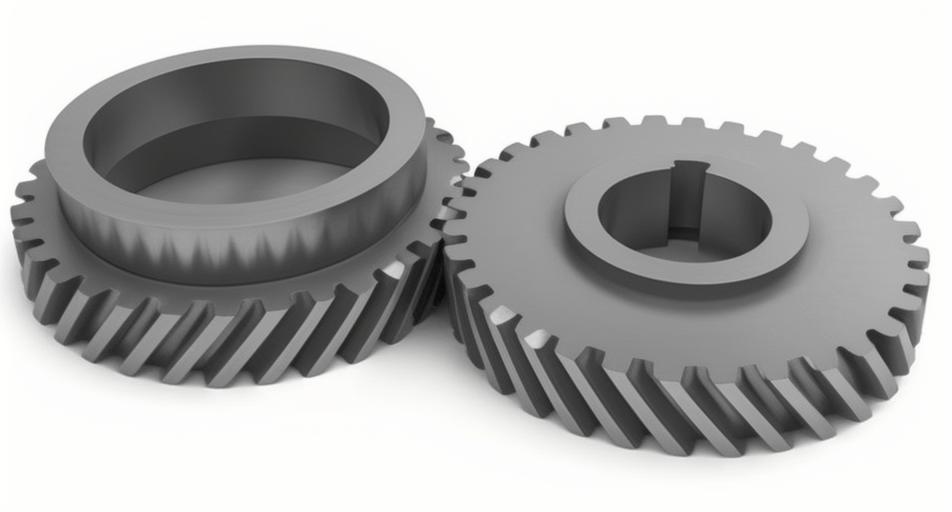
The dynamic analysis of gear transmission systems is fundamental to the design of modern high-performance machinery, where stability, efficiency, and low noise are paramount. Among various gear types, helical gears are widely preferred for their superior load capacity and smoother, quieter operation compared to spur gears, owing to their gradual tooth engagement. However, the inherent nonlinearities in helical gears systems—primarily time-varying mesh stiffness, damping, and most critically, backlash—can induce complex dynamic responses including periodic, quasi-periodic, and chaotic motions, as well as the coexistence of multiple stable states. Understanding these nonlinear phenomena, particularly the non-smooth bifurcations arising from intermittent contact loss due to backlash, is crucial for predicting vibration thresholds, avoiding undesirable dynamics, and enhancing system reliability. This article presents a comprehensive nonlinear dynamic analysis of a single-stage helical gears pair, employing numerical continuation and cell mapping techniques to unravel the intricate effects of system parameters like backlash and excitation frequency. The focus is on characterizing bifurcation sequences, identifying the mechanisms behind multi-attractor coexistence, and assessing their stability, providing a theoretical foundation for the optimal design of helical gears transmissions.
1. Mathematical Modeling of the Helical Gear System
The system under consideration is a single-stage parallel-axis helical gears pair. A lumped-parameter model is adopted, representing the pinion and gear as inertia disks connected by a nonlinear spring-damper element along the line of action. The model incorporates the essential nonlinearities: periodic mesh stiffness, linear viscous damping, static transmission error excitation, and a piecewise-linear backlash function.
1.1 Governing Equations of Motion
Using Newton’s second law, the torsional dynamics of the pinion and gear are described by:
$$I_1 \ddot{\psi}_1 + r_{b1} \cos\beta \left[ C_m (\dot{x}) + K_m(t) f(x) \right] = T_1$$
$$I_2 \ddot{\psi}_2 – r_{b2} \cos\beta \left[ C_m (\dot{x}) + K_m(t) f(x) \right] = -T_2$$
where $I_i$, $\psi_i$, $r_{bi}$ $(i=1,2)$ are the mass moments of inertia, angular displacements, and base circle radii of the pinion (1) and gear (2), respectively. $\beta$ is the helix angle, $C_m$ is the mesh damping coefficient, $K_m(t)$ is the time-varying mesh stiffness, $T_1$ is the input torque, and $T_2$ is the load torque. The relative displacement along the line of action, accounting for the static transmission error $e(t)$, is defined as:
$$x = r_{b1} \psi_1 – r_{b2} \psi_2 – e(t)$$
Its derivative is $\dot{x} = r_{b1} \dot{\psi}_1 – r_{b2} \dot{\psi}_2 – \dot{e}(t)$. The mesh force consists of a linear damping force and a nonlinear elastic force governed by the backlash function $f(x)$.
By subtracting the two equations and substituting the relative coordinate $x$, the system is reduced to a single degree-of-freedom model:
$$m_e \ddot{x} + C_m \cos\beta \ \dot{x} + K_m(t) \cos\beta \ f(x) = F_m + m_e \ddot{e}(t)$$
The equivalent mass $m_e$ is given by $m_e = I_1 I_2 / (I_1 r_{b2}^2 + I_2 r_{b1}^2)$. The mean static force is $F_m = T_1 / (r_{b1} \cos\beta) = T_2 / (r_{b2} \cos\beta)$. The transmission error is typically modeled as a harmonic excitation: $e(t) = E \sin(\omega_m t + \phi)$, where $\omega_m$ is the mesh frequency.
1.2 Dimensionless Form and Backlash Nonlinearity
To generalize the analysis, the equations are non-dimensionalized. Let $\omega_n = \sqrt{\bar{K}_m / m_e}$ be the average natural frequency, where $\bar{K}_m$ is the average mesh stiffness. Define the dimensionless time $\tau = \omega_n t$ and displacement $y = x / b_c$, where $b_c$ is a characteristic scale (often related to the nominal static deflection). The dimensionless equations become:
$$\ddot{y} + 2\zeta \cos\beta \ \dot{y} + \kappa(\tau) \cos\beta \ f(y) = W_m + W_e \Omega^2 \cos(\Omega \tau + \phi)$$
where:
- $\dot{()}$ and $\ddot{()}$ now denote derivatives with respect to $\tau$.
- $\zeta = C_m / (2 m_e \omega_n)$ is the dimensionless damping ratio.
- $\kappa(\tau) = K_m(\tau)/\bar{K}_m = 1 + \chi \cos(\Omega \tau)$ is the dimensionless stiffness variation ($\chi$ is the stiffness fluctuation coefficient).
- $W_m = F_m / (m_e \omega_n^2 b_c)$ is the dimensionless mean load.
- $W_e = E / b_c$ is the dimensionless error amplitude.
- $\Omega = \omega_m / \omega_n$ is the dimensionless excitation frequency ratio.
- The dimensionless backlash function $f(y)$ is defined as:
$$
f(y) =
\begin{cases}
y – b, & y > b \\
0, & -b \le y \le b \\
y + b, & y < -b
\end{cases}
$$
Here, $b = B / (2b_c)$ is the half the dimensionless backlash, and $B$ is the physical total backlash. This piecewise-linear function introduces the non-smoothness into the system, dividing the phase space into three distinct regions:
- Region I (Positive Mesh, $y > b$): Teeth are in contact on the drive side.
- Region II (Backlash, $-b \le y \le b$): Teeth are out of contact, resulting in free-flight with no elastic restoring force.
- Region III (Negative Mesh, $y < -b$): Teeth impact and contact on the reverse side (only possible under severe vibration or load reversal).
For numerical simulation, the second-order equation is cast into state-space form with $y_1 = y$ and $y_2 = \dot{y}$:
$$
\begin{aligned}
\dot{y}_1 &= y_2 \\
\dot{y}_2 &= W_m + W_e \Omega^2 \cos(\Omega \tau + \phi) – 2\zeta \cos\beta \ y_2 – \kappa(\tau) \cos\beta \ f(y_1)
\end{aligned}
$$
The system parameters used for the core analysis in this study are summarized in Table 1. The nominal geometric parameters of the helical gears pair are listed in Table 2.
| Parameter | Symbol | Nominal Value |
|---|---|---|
| Damping Ratio | $\zeta$ | 0.04 |
| Mean Load | $W_m$ | 0.15 |
| Error Amplitude | $W_e$ | 0.15 |
| Stiffness Fluctuation | $\chi$ | 0.1 |
| Helix Angle | $\beta$ | 21° |
| Backlash (Half) | $b$ | 0.2 – 0.6 (variable) |
| Excitation Frequency | $\Omega$ | 0.2 – 2.0 (variable) |
| Parameter | Pinion | Gear |
|---|---|---|
| Number of Teeth | 25 | 46 |
| Normal Module (mm) | 3 | |
| Normal Pressure Angle | 20° | |
| Helix Angle | 21° | |
| Face Width (mm) | 30 | |
2. Numerical Methods for Non-smooth System Analysis
Analyzing the dynamics of the non-smooth helical gears system requires specialized numerical techniques capable of accurately detecting transitions between motion regimes and tracking periodic solutions and their stability.
2.1 The Shooting Method and Continuation
The periodic solutions of the system are fixed points of the Poincaré map $\mathbf{P}: \mathbf{y}_0 \rightarrow \mathbf{y}(T; \mathbf{y}_0)$, where $T = 2\pi/\Omega$ is the excitation period and $\mathbf{y}_0 = [y_1(0), y_2(0)]^T$ is the initial state on a stroboscopic (period-T) section. A periodic solution satisfies $\mathbf{G}(\mathbf{y}_0) = \mathbf{P}(\mathbf{y}_0) – \mathbf{y}_0 = \mathbf{0}$.
The shooting method solves this boundary value problem using Newton-Raphson iteration:
$$\mathbf{y}_0^{(k+1)} = \mathbf{y}_0^{(k)} – \left[ \mathbf{DP}(\mathbf{y}_0^{(k)}) – \mathbf{I} \right]^{-1} \mathbf{G}(\mathbf{y}_0^{(k)})$$
where $\mathbf{DP}(\mathbf{y}_0)$ is the monodromy matrix (Jacobian of the Poincaré map), obtained by integrating the state transition matrix along with the trajectory.
Parameter continuation is employed to trace solution branches as a parameter (e.g., $\Omega$ or $b$) varies. Starting from a known solution $\mathbf{y}_0(\mu_0)$ at parameter $\mu_0$, a predictor step (e.g., tangent predictor) estimates the solution at $\mu_0 + \Delta\mu$, which is then corrected using the shooting method. This process reveals branches of periodic orbits, including unstable ones, which are essential for understanding global bifurcations.
2.2 Stability and Bifurcation Analysis via Floquet Theory
The stability of a periodic orbit is determined by the eigenvalues $\lambda_i$ (Floquet multipliers) of the monodromy matrix $\mathbf{DP}$. For a damped mechanical system:
- Stable periodic orbit: All multipliers lie inside the unit circle ($|\lambda_i| < 1$).
- Saddle-node (SN) bifurcation: A multiplier crosses the unit circle at +1. This creates or annihilates a pair of periodic orbits (one stable, one unstable).
- Period-doubling (PD) bifurcation: A multiplier crosses at -1. This leads to the birth of a period-$2T$ orbit.
- Neimark-Sacker (NS) bifurcation: A complex conjugate pair crosses the unit circle, leading to quasi-periodic motion.
In non-smooth systems, grazing bifurcations occur when a periodic orbit becomes tangent to (grazes) a discontinuity boundary (e.g., $y = \pm b$). This can lead to a sudden and drastic change in the system’s topology and stability. Of particular interest are compound bifurcations like grazing-saddle-node (GR-SN) bifurcations, where a saddle-node and a grazing event coincide, playing a pivotal role in the creation and destruction of attractors.
2.3 Basin of Attraction and Cell Mapping
To investigate the coexistence of multiple attractors, the basin of attraction for each stable solution must be characterized. The cell mapping method discretizes a region of interest in the phase space ($y_1$, $y_2$) into a grid of cells. Each cell is treated as a state, and a mapping determines the destination cell after one excitation period $T$. By iterating this process, cells are categorized based on the attractor they converge to, revealing the basin structure. This method is computationally efficient for visualizing the complex, often fractal boundaries between basins in nonlinear systems like helical gears with backlash.
3. Global Dynamics: Influence of Backlash and Excitation Frequency
3.1 Effect of Backlash Magnitude
The dimensionless half-backlash $b$ is a critical design parameter. Figure 1 shows multi-initial-condition bifurcation diagrams and the corresponding largest Lyapunov exponent (TLE) spectra for two different backlash values, $b=0.2$ and $b=0.6$, with $\Omega$ as the bifurcation parameter. Positive TLE indicates chaotic motion.
For moderate backlash ($b=0.2$): The system exhibits a primarily periodic response over a wide frequency range. Key bifurcations include saddle-node (SN) bifurcations near $\Omega \approx 0.62, 0.69, 0.88, 0.92$, causing jumps between different periodic-1 (P-1) solutions. A period-doubling (PD) bifurcation at $\Omega \approx 1.11$ initiates a period-2 (P-2) window, which persists until $\Omega \approx 1.59$. A narrow band of chaos appears around $\Omega \approx 1.59-1.65$, followed by a period-4 (P-4) window, an inverse period-doubling cascade back to P-2, and finally a reverse bifurcation to a stable P-1 motion for $\Omega > 1.94$.
For larger backlash ($b=0.6$): The dynamic landscape becomes significantly more complex. The chaotic region widens substantially ($\Omega \approx 1.32-1.82$). The hysteresis regions (indicative of coexisting attractors) become more pronounced, especially within the P-2 window ($\Omega \approx 1.11-1.32$), where two different P-2 attractors and a P-4 attractor can coexist depending on initial conditions. New periodic windows, such as a prominent P-4 window following the chaotic zone, emerge. The sequence of SN bifurcations at lower frequencies ($\Omega < 0.7$) also shifts and multiplies.
Conclusion: Increasing backlash in helical gears systems amplifies nonlinear effects, destabilizing the response. It expands the parameter regions associated with chaos, hysteresis, and multi-periodic motions. This underscores the importance of minimizing backlash within functional limits during the design and assembly of helical gears transmissions to enhance operational stability and reduce vibration/noise.
3.2 Bifurcation Analysis and Coexisting Attractors
To unravel the complex bifurcation structure and the evolution of coexisting attractors revealed in the global diagrams, numerical continuation is applied for the case of $b=0.6$. The resulting bifurcation diagram, tracking both stable and unstable periodic orbits, is shown in Figure 2. Orbits are labeled as “$n$-$p$-$q$”, where $n$ is the period multiplicity relative to the excitation period $T$, and $p$ and $q$ are the number of impacts with the boundaries $y=b$ and $y=-b$ per fundamental period, respectively.
The system originates as a simple non-impacting P-1 (1-0-0) motion at very low $\Omega$. As $\Omega$ increases, the following key events occur:
- Grazing Bifurcation (GR1): At $\Omega_{GR1}$, the 1-0-0 orbit grazes the $y=b$ boundary, transforming into a impacting P-1 orbit (1-1-0).
- Saddle-Node and Grazing-Saddle-Node Bifurcations: The 1-1-0 orbit loses stability via a saddle-node bifurcation (SN1). Subsequently, at $\Omega_{GR2-SN2} \approx 0.512$, a grazing-saddle-node (GR-SN) bifurcation occurs. This compound event restores stability and transforms the orbit into a double-sided impacting orbit (1-1-1).
- Period-Doubling Cascade to Chaos: The stable 1-1-0 orbit (regained after another GR-SN event) undergoes a period-doubling bifurcation (PD1) at $\Omega \approx 1.106$, leading to a P-2 orbit (2-2-0). This P-2 orbit undergoes further grazing and period-doubling events (e.g., GR4, PD2), eventually initiating a period-doubling route to chaos around $\Omega \approx 1.22$.
- Crisis and Inverse Cascade: The chaotic attractor undergoes a boundary crisis and is replaced by a P-4 window. Through a sequence of inverse period-doubling bifurcations (e.g., PD5, PD6), the system reverts to a stable P-1 (1-1-0) motion at high $\Omega$.
Coexistence Intervals: Two major intervals of multi-attractor coexistence are identified:
Interval A ($\Omega \approx [0.567, 0.689]$): Coexistence of three P-1 attractors: the original 1-0-0, the 1-1-1, and the 1-1-0, along with an unstable U1-1-0 saddle.
Interval B ($\Omega \approx [1.058, 1.308]$): Coexistence of a P-2 attractor (2-1-0 or 2-2-0), a P-4 attractor (4-2-0), and unstable saddles (U2-1-0, U2-1-1).
This analysis reveals that the dynamics of helical gears systems in the primary resonance region are governed by an intricate interplay of smooth bifurcations (SN, PD) and non-smooth bifurcations (GR, GR-SN). The GR-SN bifurcations are particularly significant as they directly mediate transitions between different types of impacting periodic motions and alter the system’s stability landscape.
3.3 Stability and Basin Evolution
The practical implication of attractor coexistence is that the final steady-state depends on the initial conditions. Using the cell mapping method, the basins of attraction are computed for selected frequencies within the coexistence intervals. The evolution of these basins elucidates the stability of each attractor.
In Interval A ($\Omega = 0.56, 0.61, 0.65$): The basins for the 1-0-0 (blue) and 1-1-1 (cyan) attractors are intricately interwoven, with fractal boundaries. The unstable U1-1-0 saddle lies on the boundary separating these basins. As $\Omega$ increases from 0.56 to 0.65:
- The basin of the 1-0-0 attractor shrinks progressively.
- The basin of the 1-1-1 attractor also contracts and becomes more fragmented.
- The basin of the 1-1-0 attractor (yellow), born from the GR-SN bifurcation, emerges and expands, indicating its growing dominance.
At $\Omega_{GR1}$, the 1-0-0 basin vanishes (grazing bifurcation). At $\Omega_{SN3}$, the 1-1-1 attractor collides with its unstable counterpart and disappears via a saddle-node bifurcation.
In Interval B ($\Omega = 1.20, 1.22, 1.24$): The basins correspond to the P-2 (yellow/green) and P-4 (dark green) attractors. The structure remains complex but shows a consistent trend:
- The basin area of the P-2 attractor gradually decreases with increasing $\Omega$.
- The basin area of the P-4 attractor expands, signifying a transfer of stability.
The unstable periodic orbits (U2-1-0, U2-1-1) form the skeletal structure of the basin boundaries.
Key Insight: The grazing-saddle-node (GR-SN) bifurcation has a profound impact on the global stability landscape. It not only changes the topological type of an orbit but also triggers a significant redistribution of the basins of attraction, potentially making previously dominant attractors vulnerable to small perturbations. In contrast, a simple grazing (GR) bifurcation, while altering the orbit’s impact pattern, may not drastically reconfigure the basin structure in the immediate parameter vicinity.
4. Discussion and Engineering Implications
The nonlinear dynamic analysis of helical gears systems presented here highlights several critical aspects for design and operation:
- Backlash Management: Backlash is a necessary evil in gear systems, but its magnitude must be tightly controlled. The results quantitatively demonstrate that even within a functionally acceptable range, increasing backlash can precipitate complex dynamics—chaos and hysteresis—that are detrimental to positioning accuracy, load sharing, and fatigue life. Precision helical gears assemblies should aim for the minimal backlash permissible by manufacturing and thermal expansion constraints.
- Frequency Operation Windows: The system exhibits rich, potentially hazardous dynamics (chaos, co-existing attractors) in specific frequency bands, particularly around and below the primary resonance ($\Omega \sim 1$). Operating a helical gears drive within these “danger zones” should be avoided or passed through quickly during run-up/down. If operation near resonance is unavoidable, increasing damping ($\zeta$) can help suppress nonlinear instabilities.
- Robustness and Safety Margins: The phenomenon of coexisting attractors implies that under identical operating conditions ($\Omega$, load), the system can settle into drastically different vibration states (e.g., low-amplitude P-1 vs. high-amplitude chaotic motion) depending on transient events like startup shocks or load fluctuations. Design should account for this by ensuring that the desired operating point lies within a large, robust basin of attraction, providing immunity against accidental crossing of fractal basin boundaries.
- Diagnostics and Modeling: The identified bifurcation sequences—especially the signature of GR-SN events—can serve as fingerprints in vibration-based condition monitoring. Abnormal shifts in these bifurcation points could indicate changes in backlash due to wear, or variations in mesh stiffness from cracks, providing a model-based approach to fault diagnosis in helical gears transmissions.
5. Conclusion
This investigation provides a detailed exploration of the non-smooth nonlinear dynamics in a single-stage helical gears transmission system. Through a combination of numerical simulation, parameter continuation, and basin stability analysis, the profound influence of backlash and excitation frequency on the system’s behavior has been elucidated. Key findings include:
- Increasing the dimensionless backlash significantly exacerbates nonlinear effects, leading to expanded regions of chaotic response, pronounced hysteresis, and the emergence of additional periodic windows, thereby degrading system stability.
- The dynamic response in the low-frequency region, particularly around primary resonance, is exceptionally rich, featuring sequences of saddle-node, period-doubling, and grazing bifurcations. Special non-smooth events like the grazing-saddle-node (GR-SN) bifurcation play a pivotal role in mediating transitions between different impacting motions and altering stability.
- The system exhibits robust intervals of multi-attractor coexistence, where multiple stable periodic orbits (e.g., P-1, P-2, P-4) exist simultaneously. The evolution of their basins of attraction reveals that GR-SN bifurcations cause major restructuring of these basins, critically affecting the system’s robustness to perturbations, whereas simple grazing bifurcations have a more localized effect.
These insights underscore the importance of considering detailed nonlinear dynamic analysis during the design phase of helical gears systems. By strategically selecting parameters to avoid dangerous bifurcation zones and ensuring operation within a robust basin of a desirable attractor, engineers can significantly enhance the performance, reliability, and longevity of gear-driven machinery. Future work could extend this model to include more degrees of freedom (e.g., lateral shaft motions), non-linear damping, and the effects of profile modifications to develop even more comprehensive design guidelines for advanced helical gears applications.