
I began my study of noncircular gear manufacturing from a practical observation: many machines require a nonlinear input–output relationship, and a pair of noncircular gears can provide that relationship with a compact, reliable, and highly efficient mechanical transmission. Unlike a standard cylindrical gear, a noncircular gear has a pitch curve whose radius changes with the polar angle. This single geometric fact changes almost every aspect of design, kinematics, interpolation, process planning, and numerical control. In my research I concentrated on the key technology of gear hobbing for noncircular gears, because gear hobbing offers high productivity, good tooth-surface quality, simple tool geometry, and strong potential for generating both straight and helical noncircular gears. I treated gear hobbing not as a simple extension of cylindrical gear cutting but as a coupled multi-axis generation process in which the tool and workpiece must maintain a continuously changing conjugate relationship.
My work had four main objectives. First, I wanted to establish accurate multi-axis kinematic models for noncircular gear hobbing, including four-axis and five-axis configurations for straight and helical gears. Second, I wanted to develop interpolation methods that can follow the noncircular pitch curve without excessive velocity fluctuation. Third, I wanted to improve the process technology of noncircular gear hobbing, especially tool path planning, automatic tool setting, cutting-parameter selection, and optimization. Fourth, I wanted to build a complete computer numerical control system that allows an operator to input gear parameters and obtain automatic gear hobbing without manual programming. The following sections summarize my models, formulas, tables, simulations, and system implementation.
The transmission principle of a noncircular gear pair can be expressed by a pitch curve. If the polar radius is a function of the polar angle, then the local tangent direction, the pressure angle at the pitch point, and the instantaneous center distance all vary. I used the following basic relations throughout my analysis:
$$ r = r(\theta) $$
$$ \tan\psi = \frac{r}{dr/d\theta} $$
$$ R = r\sin\psi = \frac{r^2}{\sqrt{r^2+(dr/d\theta)^2}} $$
$$ \phi = \theta + \psi – \theta_0 – \psi_0 $$
Here, \(r\) is the polar radius, \(\theta\) is the polar angle, \(\psi\) is the angle between the polar radius and the tangent to the pitch curve, \(R\) is the distance from the gear center to the projection of the pitch point on the machine axis, and \(\phi\) is the angular position of the workpiece. These quantities define the instantaneous geometry of gear hobbing for a noncircular gear. Because \(r\) and \(dr/d\theta\) are not constant, the center distance, the workpiece rotation, and the hob rotation cannot be linked by a fixed ratio. This is the central difficulty of noncircular gear hobbing.
I treated the hob as a moving rack cutter. In conventional gear hobbing, the hob and the gear obey a generating motion similar to a rack and a gear in mesh. For a noncircular gear, the rack cutter must roll without slipping along the noncircular pitch curve. Therefore, the instantaneous rolling arc length and the rack displacement must be equal. I used the arc-length integral
$$ S(\theta)=\int_{\theta_0}^{\theta}\sqrt{r^2+(dr/d\theta)^2}\,d\theta $$
to relate the rack displacement to the workpiece rotation. This arc-length relation is the foundation of all my kinematic models for noncircular gear hobbing.
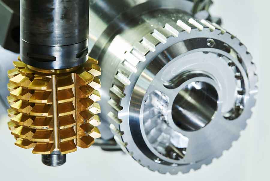
The following image illustrates the general configuration of gear hobbing that I used as the basis for my models.
In my four-axis model for straight noncircular gear hobbing, I considered four coordinated motions: workpiece rotation, hob rotation, center-distance motion, and axial feed along the workpiece axis. The axial feed mainly determines the tooth width and does not alter the instantaneous generating relation. Therefore, the core generating model consists of workpiece rotation, hob rotation, and center-distance motion. I defined the axes as follows:
| Axis | Motion | Function in gear hobbing |
|---|---|---|
| C | Workpiece rotation | Indexing and generation of the noncircular pitch curve |
| B | Hob rotation | Cutting and rack translation |
| X | Center-distance motion | Maintains rolling contact for changing pitch radius |
| Z | Axial feed | Generates the full face width |
For the four-axis model, I derived the following position relations. For any meshing point \(i\),
$$ R_i=\frac{r_i^2}{\sqrt{r_i^2+(dr/d\theta)_i^2}} $$
$$ \phi_i=\theta_i+\arctan\frac{r_i}{(dr/d\theta)_i}-\theta_0-\arctan\frac{r_0}{(dr/d\theta)_0} $$
$$ \alpha_i=\frac{2}{q m_0}\left[\int_{\theta_0}^{\theta_i}\sqrt{r^2+(dr/d\theta)^2}\,d\theta+w_i-w_0\right] $$
where \(q\) is the number of hob threads, \(m_0\) is the hob module, \(\alpha_i\) is the hob rotation angle, and \(w_i\) is the distance from the pitch point to the machine axis. The corresponding velocity relations can be written symbolically as
$$ \omega_w=\omega_t\,f_w\left(r,\frac{dr}{d\theta},\theta\right) $$
$$ v_R=\omega_t\,f_R\left(r,\frac{dr}{d\theta},\frac{d^2r}{d\theta^2},\theta\right) $$
These equations show that even when the hob rotates at a constant speed, the workpiece speed and the center-distance speed fluctuate periodically. In my simulations, this fluctuation was strongest near the minimum and maximum polar radii. The fluctuation is an inherent property of noncircular gear hobbing, not a programming error.
The four-axis model is efficient, but it has a serious limitation: the hob must move along the workpiece axis while the generating motion is active, and the actual hob length is finite. In many cases the required rack displacement is greater than the usable length of the hob. To solve this problem, I developed a five-axis model. The fifth axis is an additional axial shift of the hob along its own axis. This axial shift changes the active thread region of the hob and effectively extends the usable tool length. I derived the five-axis model by combining the rolling arc length, the hob axial shift, and the center-distance variation. The main velocity relations can be summarized as
$$ v_x=\frac{r^2+2r(dr/d\theta)^2-r^2(d^2r/d\theta^2)}{(r^2+(dr/d\theta)^2)^{3/2}}\,\omega $$
$$ v_y=\frac{r^2(dr/d\theta)+2r(dr/d\theta)^3-r^3(dr/d\theta)(d^2r/d\theta^2)}{(r^2+(dr/d\theta)^2)^{3/2}}\,\omega $$
$$ \omega_t=\frac{2}{q m_0}\sqrt{r^2+(dr/d\theta)^2}\,\omega $$
where \(v_x\) is the rack-projected axial velocity, \(v_y\) is the center-distance velocity, and \(\omega\) is the polar-angle rate. The five-axis model gives a wider working range, more uniform hob wear, and better control of the tooth-generation process. I found that the five-axis configuration is especially useful when the noncircular gear has a large eccentricity or a high order, because the required rack travel becomes large.
I also extended the models to helical noncircular gears. In helical gear hobbing, the hob axis is inclined relative to the workpiece axis, and an additional differential motion is needed. For the four-axis helical model, the workpiece rotation is related to the hob rotation by the instantaneous equivalent tooth number and the helix angle. I used the relation
$$ \omega_c=\frac{K M_n}{2 R\cos\lambda}\,\omega_b $$
where \(K\) is the number of hob starts, \(M_n\) is the normal module, \(\lambda\) is the helix angle, and \(R\) is the instantaneous center distance. The axial feed also introduces a differential rotation
$$ \Delta\omega_c=\frac{v_z\tan\lambda}{r} $$
so that the final workpiece speed is
$$ \omega_c^*=\omega_c+\Delta\omega_c $$
For the five-axis helical model, I added the hob axial shift and obtained a complete set of coupled equations. These equations are more complex than those for straight gears, but they are necessary when the helix angle is large or when the hob must be shifted to avoid localized wear. I summarized the differences between the straight and helical models in the following table.
| Model | Number of axes | Main additional relation | Typical use |
|---|---|---|---|
| Straight four-axis gear hobbing | 4 | Center-distance variation and constant-ratio hob–workpiece motion | General straight noncircular gears |
| Straight five-axis gear hobbing | 5 | Hob axial shift for long rack travel | Large eccentricity or long pitch curve |
| Helical four-axis gear hobbing | 4 | Differential motion from helix angle and axial feed | Small helix angle helical noncircular gears |
| Helical five-axis gear hobbing | 5 | Combined differential and hob axial shift | Large helix angle and long face width |
Once the kinematic models were established, I turned to interpolation. The pitch curve of a noncircular gear is a smooth curve, but a numerical control system cannot directly execute an arbitrary analytic curve. The curve must be discretized into small segments, and the motion axes must be commanded at each interpolation period. The choice of discretization method strongly affects accuracy, speed fluctuation, and machine vibration. I studied two discretization principles: equal polar angle and equal arc length. I also studied two interpolation types: linear interpolation and spline interpolation. The combinations produce four practical methods for noncircular gear hobbing.
In equal-polar-angle discretization, the polar angle is divided into equal increments:
$$ \Delta\theta=\frac{2\pi}{N} $$
The corresponding pitch points are
$$ \theta_k=k\Delta\theta,\qquad r_k=r(\theta_k) $$
This method is simple and fast. However, because the arc length per increment changes with the local radius, the points become dense near the minimum and maximum radii and sparse in the middle regions. In gear hobbing, dense points mean that the tool spends more time in those regions, which can change the local tooth-surface finish and tool load.
In equal-arc-length discretization, the arc length is divided into equal increments:
$$ \Delta S=\frac{S_{\max}}{N} $$
For each increment, the next polar angle must satisfy
$$ \int_{\theta_k}^{\theta_{k+1}}\sqrt{r^2+(dr/d\theta)^2}\,d\theta=\Delta S $$
This equation is a transcendental equation. I solved it by the Newton–Raphson method:
$$ \theta_{k+1}^{(j+1)}=\theta_{k+1}^{(j)}-\frac{F(\theta_{k+1}^{(j)})}{F'(\theta_{k+1}^{(j)})} $$
where
$$ F(\theta)=\int_{\theta_k}^{\theta}\sqrt{r^2+(dr/d\theta)^2}\,d\theta-\Delta S $$
The integral was evaluated by the composite Simpson rule:
$$ \int_a^b f(x)\,dx\approx\frac{h}{3}\left[f(a)+f(b)+4\sum_{i=1}^{m}f(x_{2i-1})+2\sum_{i=1}^{m-1}f(x_{2i})\right] $$
Equal-arc-length discretization gives a more uniform distribution of generating points along the pitch curve. It reduces local over-cutting and under-cutting in noncircular gear hobbing, but it requires more computation. I implemented the method in MATLAB and verified the arc-length integral against an analytic test function. The numerical error was on the order of \(10^{-6}\) for a moderate number of subdivisions, which is acceptable for practical gear hobbing.
For the interpolation itself, I first considered linear interpolation. If two adjacent pitch points are known, the tool path between them is approximated by a straight line. Linear interpolation is easy to implement and is supported by almost every numerical control system. However, it produces piecewise-constant velocity and discontinuous acceleration. In noncircular gear hobbing, this causes periodic impacts and may excite structural vibration. The interpolation error decreases as the number of segments increases, but the number of program blocks also increases. I found that linear interpolation can be used for rough gear hobbing when the required accuracy is not very high.
To improve smoothness, I developed a cubic B-spline interpolation method for noncircular gear hobbing. I represented each segment of the pitch curve as
$$ x(u)=A_0+A_1u+A_2u^2+A_3u^3 $$
$$ y(u)=B_0+B_1u+B_2u^2+B_3u^3 $$
$$ P(u)=(x(u),y(u)),\qquad u\in[0,1] $$
The arc-length derivative is
$$ \frac{ds}{du}=\sqrt{\left(\frac{dx}{du}\right)^2+\left(\frac{dy}{du}\right)^2} $$
For a commanded feed rate \(f\) and interpolation period \(T\), the parameter increment is obtained from
$$ \Delta u_i=\frac{fT}{\sqrt{x’^2+y’^2}} -\frac{x’x”+y’y”}{2(x’^2+y’^2)^2}(fT)^2 $$
The next parameter value is
$$ u_{i+1}=u_i+\Delta u_i $$
and the next interpolation point is
$$ P_{i+1}=P(u_{i+1}) $$
I converted this point into polar coordinates:
$$ r_{i+1}=\sqrt{x_{i+1}^2+y_{i+1}^2} $$
$$ \theta_{i+1}=\arctan\frac{y_{i+1}}{x_{i+1}} $$
Then I used the kinematic models to compute the motion increments for each axis in gear hobbing. The spline method provides continuous velocity and smoother acceleration than linear interpolation. It is particularly effective for the center-distance axis, which reverses direction at the minimum and maximum radii. With linear interpolation, this reversal produces a sharp velocity jump. With spline interpolation, the reversal is rounded and the dynamic load on the ball screw is reduced.
I compared four interpolation strategies for noncircular gear hobbing: equal-polar-angle with linear interpolation, equal-polar-angle with spline interpolation, equal-arc-length with linear interpolation, and equal-arc-length with spline interpolation. I used a third-order elliptical gear with a long-axis radius of \(150\,\text{mm}\), an eccentricity of \(0.1\), and a module of \(2.5\). The hob had two starts and rotated at \(200\,\text{r/min}\). The results are summarized below.
| Interpolation method | Maximum error for 200 points | Maximum error for 300 points | Velocity smoothness | Computational load |
|---|---|---|---|---|
| Equal polar angle + linear | 0.020 mm | 0.00905 mm | Poor; sawtooth fluctuation | Low |
| Equal polar angle + spline | 0.00071 mm | Lower than linear | Good near mid-radius; moderate near extremes | Medium |
| Equal arc length + linear | About 0.018 mm | 0.00792 mm | Better than equal polar angle; still sawtooth | Medium |
| Equal arc length + spline | Lowest | Lowest | Best; smooth periodic variation | High |
The simulation showed that spline interpolation greatly reduces the interpolation error. At 200 discrete points, the maximum spline error was \(7.1\times10^{-4}\,\text{mm}\), while the linear error was about \(0.02\,\text{mm}\). At 300 points, the linear error dropped to \(9.05\times10^{-3}\,\text{mm}\), but it remained an order of magnitude larger than the spline error. The equal-arc-length spline method gave the best overall accuracy and the smoothest axis motion. However, it also required the most computation and placed the highest demand on the controller. I concluded that the equal-arc-length spline method is best for finishing gear hobbing, while the equal-arc-length linear method is a reasonable compromise for rough gear hobbing.
I also simulated the axis speeds. The workpiece speed varied periodically with the polar angle. It was highest at the minimum polar radius and lowest at the maximum polar radius. The center-distance speed was zero at the minimum and maximum radii and reached its peak at intermediate radii. With linear interpolation, both speeds showed high-frequency fluctuations. With spline interpolation, the speeds were smooth and periodic. The hob speed also showed a periodic component when the hob was not chosen as the master axis. In my control strategy, I usually set the hob as the master axis and let the workpiece and center-distance axes follow. This reduces hob wear and simplifies the spindle control, but it transfers the speed fluctuation to the workpiece and center-distance axes. Therefore, the dynamic characteristics of those axes must be considered in process optimization.
After the kinematic and interpolation models were established, I studied the process technology of noncircular gear hobbing. The first issue was the tool path. I selected axial gear hobbing as the main cutting method because it is widely used and produces good tooth-surface quality. In axial gear hobbing, the hob moves along the workpiece axis while the generating motion continues. The tool path includes a rapid approach, a feed to the cutting position, the cutting stroke, a retract, and a rapid return. I defined the path by a sequence of coordinates. The cutting start point, the cutting end point, and the safe retract point were calculated from the gear width, the hob radius, and the depth of cut. A typical path can be described as
$$ X_2=X_A-r+\Delta f $$
$$ Z_2=Z_A+\frac{\Delta f}{\cos\theta} $$
$$ X_3=X_2+100 $$
$$ Z_3=Z_2 $$
$$ X_4=X_3 $$
$$ Z_4=Z_3-B $$
$$ X_5=X_4+100 $$
$$ Z_5=Z_4 $$
where \(X_A\) and \(Z_A\) are the coordinates of the initial contact point, \(r\) is the hob radius, \(\Delta f\) is the depth of cut, \(B\) is the face width, and \(\theta\) is the hob setting angle. This path keeps the hob clear of the workpiece during rapid motions and ensures that the generating motion is fully established before the cut begins.
The second process issue was tool setting. Noncircular gears have a specific meshing reference position. The zero line of the driving gear must be located at a tooth groove center when the zero line of the driven gear is located at a tooth center. If the initial angular position is wrong, the gear pair will not mesh correctly. Manual tool setting is slow and inaccurate. I proposed an automatic tool-setting method using absolute photoelectric encoders on both the hob axis and the workpiece axis. The hob zero position was defined at a specified tooth tip or tooth space center. The workpiece zero position was defined by a pin hole on the worktable and the worktable rotation center. When both encoders reached their zero positions, the initial angular alignment was established. The X and Z coordinates were then recorded at the contact point and converted into the workpiece zero point by
$$ X_A=X_P-r $$
$$ Z_A=Z_P-r $$
where \(X_P\) and \(Z_P\) are the recorded contact coordinates. This method improved both the accuracy and the repeatability of tool setting in noncircular gear hobbing.
The third process issue was cutting-parameter selection. In cylindrical gear hobbing, cutting speed, feed rate, depth of cut, number of passes, and finishing allowance are usually selected from handbook tables or workshop experience. For noncircular gear hobbing, those tables are not directly applicable because the cutting speed and the material removal rate vary along the pitch curve. I therefore developed an optimization model for cutting parameters. I used the maximum average profit rate as the objective function:
$$ \max P=\frac{S-C}{T} $$
where \(S\) is the selling price of one gear, \(C\) is the production cost of one gear, and \(T\) is the production time of one gear. The production time included cutting time, tool-change time, and auxiliary time:
$$ T=t_q+\frac{t_q}{T_d}t_t+t_s $$
The tool life was modeled as
$$ T_d=C_r v^r f^q a_p^l $$
The production cost included material cost, labor cost, and tool-change cost:
$$ C=M+C_m t_q+C_t\frac{t_q}{T_d} $$
Combining these relations gave the objective function
$$ \max P=\frac{S-M-C_m t_q-C_t t_q/T_d}{t_q+t_q t_t/T_d+t_s} $$
I then imposed constraints from the machine tool, the cutting tool, the workpiece quality, and the transmission components. The main constraints were
$$ f_{\min}\le f\le f_{\max} $$
$$ v_{\min}\le v\le v_{\max} $$
$$ P_c\le \eta P_{\max} $$
$$ R_a=\frac{0.0321 f^2}{r_a}\le R_{a\max} $$
$$ F_d=m’a+\mu m’g\le F_{\max} $$
$$ Q=\frac{n k}{60}\le Q_{\max} $$
where \(f\) is feed, \(v\) is cutting speed, \(P_c\) is cutting power, \(\eta\) is machine efficiency, \(P_{\max}\) is the maximum spindle power, \(R_a\) is surface roughness, \(r_a\) is the hob tip radius, \(F_d\) is the dynamic load on the ball screw, \(m’\) is the mass of the hob slide, \(a\) is its acceleration, \(\mu\) is the friction coefficient, \(F_{\max}\) is the maximum allowable load, \(Q\) is the cutting-force fluctuation frequency, \(n\) is the hob speed, and \(k\) is the number of hob teeth. The acceleration of the center-distance axis was obtained by differentiating the center-distance velocity from the kinematic model. This constraint is unique to noncircular gear hobbing because the center-distance axis must accelerate and decelerate continuously as the pitch radius changes.
I solved the constrained optimization problem with a particle swarm optimization algorithm. The objective function was converted into an unconstrained penalized function:
$$ \Phi(v,f)=P(v,f)-\epsilon\sum_{i=1}^{8}u_i g_i(v,f) $$
where \(\epsilon\) is a penalty factor and \(u_i\) is a penalty indicator. The particle swarm update equations were
$$ v_i^{j+1}=w v_i^j+c_1 r_1(p_i-x_i^j)+c_2 r_2(u-x_i^j) $$
$$ x_i^{j+1}=x_i^j+v_i^{j+1} $$
The inertia weight was reduced linearly:
$$ w=0.9-0.5\frac{j}{j_{\max}} $$
I used a population of 100 particles and 100 iterations. The optimization converged quickly. For a typical noncircular gear made of 45 steel, with a module of 3, a hob diameter of 80 mm, one hob start, and a helix angle of \(2^\circ\), the optimized cutting speed was about \(77.213\,\text{m/min}\) and the feed rate was about \(3.4\,\text{mm/r}\). The particle distribution contracted toward a small region after about 40 iterations, and the final solution satisfied all constraints. This showed that the particle swarm method is suitable for cutting-parameter optimization in noncircular gear hobbing, where the objective function is nonlinear and the constraints are strongly coupled.
I summarized the optimization variables, constraints, and results in the following tables.
| Variable or parameter | Symbol | Value or range |
|---|---|---|
| Spindle speed range | n | 30–2440 r/min |
| Feed range | f | 0.1–5 mm/r |
| Maximum power | Pmax | 18 kW |
| Machine efficiency | η | 0.9 |
| Maximum ball-screw load | Fmax | 142000 N |
| Hob diameter | d0 | 80 mm |
| Hob starts | q | 1 |
| Hob module | m0 | 3 mm |
| Hob helix angle | β | 2° |
| Noncircular gear order | n | 2 |
| Long-axis radius | a | 50 mm |
| Eccentricity | k | 0.2 |
| Number of teeth | z | 30 |
| Hob teeth | k | 8 |
| Constraint | Expression | Purpose |
|---|---|---|
| Feed limit | \(f_{\min}\le f\le f_{\max}\) | Protect machine feed drive |
| Speed limit | \(v_{\min}\le v\le v_{\max}\) | Protect spindle and tool |
| Power limit | \(P_c\le \eta P_{\max}\) | Prevent spindle overload |
| Roughness limit | \(R_a\le R_{a\max}\) | Ensure surface quality |
| Dynamic load limit | \(F_d\le F_{\max}\) | Protect ball screw and slide |
| Vibration limit | \(Q\le Q_{\max}\) | Avoid forced vibration |
| Optimization parameter | Value |
|---|---|
| Population size | 100 |
| Maximum iterations | 100 |
| Penalty factor | 100 |
| Learning factors | c1=c2=0.9 |
| Optimized cutting speed | 77.213 m/min |
| Optimized feed rate | 3.4 mm/r |
The final part of my research was the development of a complete numerical control system for noncircular gear hobbing. I chose an open architecture because noncircular gear hobbing requires frequent changes in gear parameters, interpolation methods, and process strategies. A closed architecture would make it difficult to implement new algorithms. I used a host–target structure. The host computer was an industrial PC running Windows XP. The target controller was a programmable multi-axis controller, PMAC, installed in the PC bus. The host computer performed system management, human–machine interaction, parameter input, program generation, and data storage. The PMAC performed real-time motion control, servo updating, interpolation, and input/output handling. The two processors communicated through a shared bus and a dynamic link library.
The hardware platform included the following components.
| Component | Function |
|---|---|
| Industrial PC | System management, interface, file storage, program generation |
| PMAC multi-axis controller | Real-time motion control, servo update, interpolation, PLC tasks |
| Servo drives and motors | Workpiece rotation, hob rotation, center-distance motion, axial feed |
| Absolute encoders | Position feedback and automatic tool setting |
| I/O modules | Coolant, limit switches, alarms, auxiliary functions |
| Communication interface | Host–target data exchange |
I mapped the machine axes to the PMAC coordinate system as follows:
$$ \#1\rightarrow 1000X $$
$$ \#2\rightarrow 1000Y $$
$$ \#3\rightarrow 1000Z $$
$$ \#4\rightarrow 1000U $$
Here, motor 1 drives the hob, motor 2 drives the workpiece, motor 3 drives the center-distance axis, and motor 4 drives the axial feed or hob shift. The scale factor 1000 converts motor counts into position units. The PMAC program used the spline mode to execute the interpolation points. A typical program segment was
$$ \text{OPEN PROG 1} $$
$$ \text{CLEAR} $$
$$ \text{SPLINE1} $$
$$ \text{INC} $$
$$ \text{TM 20000} $$
$$ \text{TA 100} $$
$$ X\ldots\;Y\ldots\;Z\ldots\;U\ldots $$
The host software was developed in Visual Basic 6.0. I used the Pcomm32 dynamic link library to communicate with the PMAC. The main interface modules were process parameters, hob parameters, workpiece parameters, tool setting, program generation, program loading, start, pause, and stop. The operator did not need to write G-code or calculate the pitch curve. The operator only entered the gear parameters, such as order, module, number of teeth, eccentricity, long-axis radius, face width, addendum, dedendum, helix angle, and hand of helix. The software then calculated the pitch curve, discretized it, generated the interpolation points, converted them into axis commands, and downloaded the program to the PMAC. This greatly reduced the programming burden and made noncircular gear hobbing accessible to operators without specialized mathematical training.
I summarized the software modules in the following table.
| Module | Input | Output or action |
|---|---|---|
| Process parameters | Speed level, depth of cut, feed, allowance | Sets cutting strategy for gear hobbing |
| Hob parameters | Module, starts, pressure angle, helix angle, outer diameter | Checks compatibility and computes hob motion |
| Workpiece parameters | Order, teeth, long-axis radius, eccentricity, width, module | Defines the noncircular pitch curve |
| Tool setting | Encoder zero, contact position | Establishes the initial meshing position |
| Program generation | All geometric and process parameters | Generates axis motion commands |
| Program loading | Generated file | Downloads commands to PMAC |
| Monitoring | Axis position, speed, status | Displays real-time data and alarms |
The PMAC controller has several features that are well suited to noncircular gear hobbing. It can execute motion programs and PLC programs simultaneously. It performs servo updates at a fixed frequency, typically 2000 Hz, and commutation updates at about 9000 Hz. It supports linear, circular, PVT, and spline interpolation modes. It provides background tasks for safety checks, watchdog timing, and error handling. It also supports real-time communication with the host computer. These features allowed me to implement a flexible and reliable control system.
I paid special attention to the dynamic behavior of the center-distance axis. In noncircular gear hobbing, this axis must follow a nonlinear function. The required acceleration can be high when the pitch curve has a large curvature change or when the gear order is high. If the acceleration exceeds the capability of the servo drive or the ball screw, the actual motion will lag behind the command. This lag causes tooth-profile error and may also excite vibration. Therefore, I included the dynamic load constraint in the cutting-parameter optimization. The acceleration of the center-distance axis was
$$ a=\frac{d}{dt}v_R=\omega^2\frac{d^2R}{d\theta^2}+\alpha\frac{dR}{d\theta} $$
where \(\alpha\) is the angular acceleration of the polar angle. When the hob is the master axis and the gear is driven at a variable speed, \(\alpha\) is not zero. This further increases the dynamic load. I found that smoothing the interpolation and limiting the cutting speed are effective ways to reduce the dynamic load. The spline interpolation method was especially helpful because it avoids abrupt changes in the velocity command.
I also considered the effect of the hob axial shift in the five-axis model. The axial shift is not a simple constant feed; it must be synchronized with the generating motion to keep the active thread region within the usable hob length. If the shift is too fast, the hob may not fully engage the tooth space. If the shift is too slow, the hob may wear unevenly. I therefore treated the axial shift as a controlled axis and included it in the interpolation. In the five-axis model, the axial shift command was calculated from the accumulated rack displacement and the current hob position. This allowed long noncircular gears to be cut with a short hob.
For verification, I simulated the complete gear hobbing process in MATLAB. I generated the pitch curve, discretized it, computed the axis commands, and plotted the motion trajectories. I also generated the PMAC program and checked it in a numerical prototype. Because the machine tool was still being commissioned, I could not perform a full cutting test on the final machine. However, I ran the same control code on a numerical prototype with equivalent motion functions. The motors rotated simultaneously, the speeds matched the predicted values, and the axis reversals occurred at the expected positions. This gave me confidence that the kinematic models, interpolation algorithms, and control system are consistent.
The main results of my research can be summarized as follows. I established four-axis and five-axis kinematic models for noncircular gear hobbing, including both straight and helical gears. I developed an equal-arc-length spline interpolation method that reduces interpolation error and smooths axis motion. I proposed an automatic tool-setting method using absolute encoders. I built a cutting-parameter optimization model that considers production time, cost, machine power, surface roughness, dynamic load, and vibration frequency, and I solved it with particle swarm optimization. I developed a host–target numerical control system for noncircular gear hobbing using an industrial PC and a PMAC controller. The system allows the operator to input gear parameters and obtain automatic gear hobbing without manual programming.
The following table gives a condensed comparison of the main technical elements of my work.
| Technical element | Method used | Main advantage | Remaining limitation |
|---|---|---|---|
| Kinematic modeling | Tool-rack method, four-axis and five-axis models | Accurate coupling of hob, workpiece, and center distance | Highly eccentric gears still require careful dynamic checks |
| Interpolation | Equal arc length, cubic spline, Newton–Raphson, Simpson | Low error and smooth velocity | Higher computational load |
| Tool path | Axial gear hobbing with rapid approach and retract | Simple and productive | Requires adequate hob length unless five-axis shift is used |
| Tool setting | Absolute encoders and pin-hole reference | Fast and repeatable | Requires encoder installation and calibration |
| Parameter optimization | Maximum profit rate, particle swarm optimization | Balances cost, time, and constraints | Model coefficients must be calibrated for different materials |
| Control system | Industrial PC + PMAC, VB6.0 interface | Open, flexible, and operator-friendly | Full machine testing still needed |
My simulations showed that the interpolation method has a strong influence on the quality of noncircular gear hobbing. With equal-polar-angle linear interpolation, the maximum error was about \(0.02\,\text{mm}\) at 200 points. With equal-arc-length spline interpolation, the error was below \(7.1\times10^{-4}\,\text{mm}\). The axis velocity curves were also much smoother with spline interpolation. The center-distance axis was the most critical axis because it must reverse direction at the minimum and maximum radii. Its acceleration was highest when the pitch curve changed rapidly. The workpiece axis also showed significant speed fluctuation, especially when the pitch radius was small. The hob axis was relatively stable when it was chosen as the master axis, but its load varied periodically because the contact length and the cutting speed changed along the pitch curve.
For process optimization, I found that the maximum profit rate is a useful objective for industrial production. It accounts for material cost, labor cost, tool cost, and production time. The tool-life equation \(T_d=C_r v^r f^q a_p^l\) was essential because it couples the cutting speed and feed rate to tool replacement. The power constraint prevented spindle overload. The surface roughness constraint ensured that the gear hobbing process could meet the finishing requirement. The dynamic load constraint protected the ball screw from excessive acceleration. The vibration frequency constraint helped avoid resonance. Because these constraints are nonlinear and sometimes conflicting, a population-based optimization method such as particle swarm optimization was more robust than a simple gradient method. The optimized parameters reduced the production cost while maintaining acceptable tool life and surface quality.
For the control system, I found that the PMAC controller is well suited to noncircular gear hobbing. Its spline mode allowed me to download a sequence of points and let the controller generate smooth motion between them. Its PLC mode allowed me to handle auxiliary functions such as coolant, limits, and alarms. Its dual-processor architecture separated the non-real-time human–machine interface from the real-time motion control. The Visual Basic interface made the system easy to use. The operator could save parameter sets, load them later, and generate a new program without recalculating the pitch curve manually. This is important because noncircular gears are often produced in small batches and the setup time must be minimized.
Nevertheless, I also identified several limitations. The interpolation algorithms were validated mainly by simulation, and their full compatibility with the PMAC spline mode was not studied in depth. The error model considered only the interpolation error and the kinematic error; it did not include thermal error, tool wear, fixture error, or servo lag. The automatic tool-setting method assumed that the encoder zero positions are stable and accurately calibrated. The optimization model used coefficients that may need to be adjusted for different workpiece materials and hob coatings. The five-axis model increased the working range but also increased the number of synchronized axes, which raises the cost and the control complexity. Finally, the machine tool was still being commissioned, so the full cutting test was not completed. These limitations define the direction for future work.
In future work, I would extend the interpolation and control algorithms to include real-time error compensation. I would build a more complete error model that includes thermal deformation, tool wear, and servo dynamics. I would study the compatibility between the host-generated spline points and the controller-native spline interpolation. I would test different noncircular gear shapes, including high-order elliptical gears, eccentric gears, and possibly concave pitch curves. I would also investigate whether the five-axis gear hobbing strategy can be extended to internal noncircular gears or to gears with very large face widths. On the process side, I would calibrate the cutting-force and tool-life coefficients for a wider range of materials. On the system side, I would improve the human–machine interface and add a simulation module so that the operator can preview the tool path and the axis motion before cutting. I would also add a database for hob parameters, workpiece materials, and successful process recipes.
Overall, my research shows that noncircular gear hobbing is a feasible and promising manufacturing method. The key is to treat the process as a coupled multi-axis generation problem, not as a simple modification of cylindrical gear hobbing. Accurate kinematic models provide the foundation. Smooth interpolation reduces dynamic error. Process optimization improves economic efficiency. An open control system makes the method practical. With further development, I believe that noncircular gear hobbing can become a standard method for producing high-quality noncircular gears for transmission systems, agricultural machinery, instruments, flow meters, and other variable-ratio applications. The combination of mathematical modeling, interpolation theory, process optimization, and open-architecture control gives a complete technical path from gear parameters to automatic gear hobbing.
In conclusion, I established a systematic framework for noncircular gear hobbing. I derived four-axis and five-axis models for straight and helical gears. I developed equal-arc-length spline interpolation and compared it with linear interpolation. I proposed automatic tool setting and cutting-parameter optimization. I built a host–target control system with an industrial PC and a PMAC controller. The simulation results confirmed that the proposed methods reduce interpolation error and smooth axis motion. The optimization results showed that the maximum profit rate can be improved while satisfying machine, tool, quality, and dynamic constraints. The control system demonstrated that an operator can generate noncircular gear hobbing programs from basic gear parameters. These results provide a solid basis for further research and industrial application of noncircular gear hobbing.