
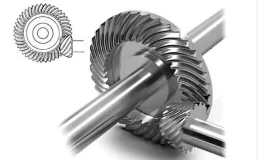
Spiral bevel gears are critical components in high-speed, heavy-duty transmission systems due to their high transmission ratio, robust load-carrying capacity, and operational stability. They are widely employed in aerospace, automotive, and precision machinery applications. Understanding the nonlinear dynamic behavior of spiral bevel gear transmission systems is essential for optimizing design, manufacturing, and operational reliability. This article comprehensively analyzes the nonlinear dynamics of spiral bevel gear systems, considering key factors such as bearing support forces, time-varying mesh stiffness, tooth side clearance, meshing damping, and static transmission errors. A dynamic model is developed, and the system’s vibrational differential equations are solved using the Runge-Kutta method. The dynamic responses under varying external excitation amplitudes are examined through time-domain diagrams, frequency-domain diagrams, phase portraits, Poincaré sections, bifurcation diagrams, wavelet time-frequency diagrams, and Lyapunov exponents. Experimental validation is conducted to verify the model’s accuracy. The results indicate that system motion transitions from chaotic to multi-periodic and finally to single-periodic states as the external excitation amplitude increases, highlighting the importance of optimal excitation levels for system stability.
Introduction
Spiral bevel gears are integral to modern mechanical systems, offering superior performance in high-load and high-speed environments. The nonlinear dynamics of spiral bevel gear transmission systems have garnered significant attention due to their complex vibrational characteristics, which arise from factors like time-varying mesh stiffness, backlash, and damping. These nonlinearities can lead to undesirable phenomena such as chaos and bifurcation, impacting system reliability and longevity. This study aims to explore the nonlinear dynamic behavior of spiral bevel gear systems through mathematical modeling, numerical simulation, and experimental validation. By investigating the effects of external excitation amplitudes on system dynamics, this research provides insights into optimizing spiral bevel gear performance and avoiding unstable operational regimes.
Dynamic Model Formulation
The dynamic model of the spiral bevel gear transmission system is developed using a lumped mass approach, where the masses of shafts are concentrated at the gear tooth width centers. The system incorporates nonlinear elements such as bearing support forces, time-varying mesh stiffness, tooth side clearance, meshing damping, and static transmission errors. The model neglects torsional vibrations and focuses on translational and rotational degrees of freedom. The generalized coordinates for the system include displacements along the X, Y, and Z axes and rotational displacements for both the driving and driven gears, as well as bearing supports.
The spiral bevel gear system’s dynamic behavior is governed by a set of nonlinear differential equations. Key parameters for the spiral bevel gears are summarized in Table 1.
| Parameters | Driving Gear | Driven Gear |
|---|---|---|
| Number of Teeth | 12 | 48 |
| Module (mm) | 5 | 5 |
| Tooth Width (mm) | 37.1 | 37.1 |
| Pressure Angle (°) | 20 | 20 |
| Helix Angle (°) | 35 | 35 |
Bearing Model
The bearing dynamics are analyzed using a circumferential line velocity method. The inner race is assumed rigidly connected to the gear shaft, rotating at the same angular velocity, while the outer race is fixed. The rolling elements are uniformly distributed, and their position angles are given by:
$$ \theta_i(t) = \frac{2\pi (i-1)}{N_b} + \frac{v_{bn} + v_{bw}}{r_{bn} + r_{bw}} t $$
where $N_b$ is the number of rolling elements, $v_{bn}$ and $v_{bw}$ are the linear velocities at contact points, and $r_{bn}$ and $r_{bw}$ are the radii of the inner and outer races. The deformation $\delta$ of the rolling elements under load is derived from Hertzian contact theory, and the bearing support forces in the X, Y, and Z directions are calculated as:
$$ F_{bx} = \sum_{i=1}^{N_b} \left[ K_b \delta^{1.5} \cos \vartheta’_i \cdot H(\delta) \right] \cos \theta_i $$
$$ F_{by} = \sum_{i=1}^{N_b} \left[ K_b \delta^{1.5} \cos \vartheta’_i \cdot H(\delta) \right] \sin \theta_i $$
$$ F_{bz} = \sum_{i=1}^{N_b} \left[ K_b \delta^{1.5} \cos \vartheta’_i \cdot H(\delta) \right] $$
Here, $K_b$ is the bearing stiffness, and $H$ is the Heaviside function. The bearing forces for the driving and driven gears under an input speed of 3000 rpm and input torque of 100 N·m are illustrated in Figure 2, showing periodic variations due to rotational dynamics.
Time-Varying Mesh Stiffness
The time-varying mesh stiffness of the spiral bevel gear is computed using the potential energy method combined with the slicing technique. Each gear tooth is divided into multiple slices along the tooth width, and each slice is treated as a spur gear. The total energy includes bending, shear, axial compression, and Hertzian contact energies, with corresponding stiffness components calculated as:
$$ \frac{1}{k_{B_j}} = \left\{ \left[ 1 – \left( \frac{z_f – 2.5}{z_f \cos \alpha_n} \right) \cos \alpha_1 \cos \alpha_3 \right]^3 – (1 – \cos \alpha_1 \cos \alpha_2)^3 \right\} / \left( 2 \Delta w E \cos \alpha_1 \sin^3 \alpha_2 \right) + \int_{-\alpha_1}^{\alpha_2} \frac{3 \{1 + \cos \alpha_1 [(\alpha_2 – \alpha) \sin \alpha – \cos \alpha]\}^2 (\alpha_2 – \alpha) \cos \alpha}{2 \Delta w E [\sin \alpha + (\alpha_2 – \alpha) \cos \alpha]^3} d\alpha $$
$$ \frac{1}{k_{S_j}} = 1.2(1 + \nu) \cos^2 \alpha_1 \left( \cos \alpha_2 – \frac{z_f – 2.5}{z_f \cos \alpha_n} \cos \alpha_3 \right) / (\Delta w E \sin \alpha_2) + \int_{-\alpha_1}^{\alpha_2} \frac{1.2(1 + \nu) (\alpha_2 – \alpha) \cos \alpha \cos^2 \alpha_1}{\Delta w E [\sin \alpha + (\alpha_2 – \alpha) \cos \alpha]} d\alpha $$
$$ \frac{1}{k_{A_j}} = \sin^2 \alpha_1 \left( \cos \alpha_2 – \frac{z_f – 2.5}{z_f \cos \alpha_n} \cos \alpha_3 \right) / (2 \Delta w E \sin \alpha_2) + \int_{-\alpha_1}^{\alpha_2} \frac{(\alpha_2 – \alpha) \cos \alpha \sin^2 \alpha_1}{2 \Delta w E [\sin \alpha + (\alpha_2 – \alpha) \cos \alpha]} d\alpha $$
$$ k_{H_j} = \frac{\pi \Delta w E}{4(1 – \nu^2)} $$
The gear foundation stiffness $k_{F_j}$ is given by:
$$ \frac{1}{k_{F_j}} = \frac{\cos^2 \alpha_m}{\Delta w E} \left[ L^* \left( \frac{\mu_F}{S_F} \right)^2 + M^* \frac{\mu_F}{S_F} + P^* (1 + Q^* \tan^2 \alpha_m) \right] $$
The overall time-varying mesh stiffness $K_h(t)$ for multiple tooth pairs in contact is:
$$ K_h(t) = \sum_{a=1}^{m} \left[ \sum_{j=1}^{n} \frac{\cos^2 \beta_m}{\frac{1}{k_{H_j}} + \frac{1}{k_{F_{jf}}} + \frac{1}{k_{B_{jf}}} + \frac{1}{k_{A_{jf}}} + \frac{1}{k_{S_{jf}}} } \right] $$
where $m$ is the number of simultaneously engaged tooth pairs, $n$ is the number of slices, and $\beta_m$ is the spiral angle at the tooth width center. The time-varying mesh stiffness exhibits periodic fluctuations, as shown in Figure 3, which influences the dynamic response of the spiral bevel gear system.
Gear Pair Relative Displacement and Meshing Force
The relative displacement along the mesh line $X_{ml}$ for the spiral bevel gear pair is expressed as:
$$ X_{ml} = (Z_1 – Z_2 + r_{m1} \theta_1 – r_{m2} \theta_2) \cos \alpha_{n1} \cos \delta_1 – (Y_1 – Y_2) (\sin \alpha_{n1} \sin \delta_1 + \cos \alpha_{n1} \sin \beta_m \cos \delta_1) + (X_2 – X_1) (\sin \alpha_{n1} \cos \delta_1 – \cos \alpha_{n1} \sin \beta_m \sin \delta_1) – e_n(t) $$
Here, $r_{m1}$ and $r_{m2}$ are the mesh radii, $\alpha_{n1}$ is the normal pressure angle, $\beta_m$ is the spiral angle, $\delta_1$ is the pitch cone angle, and $e_n(t)$ is the static transmission error. The tooth side clearance is modeled using a piecewise function:
$$ f(X_{ml}) = \begin{cases}
X_{ml} – b_m, & X_{ml} > b_m \\
0, & |X_{ml}| \leq b_m \\
X_{ml} + b_m, & X_{ml} < -b_m
\end{cases} $$
The meshing force along the mesh line and its components in the X, Y, and Z directions are:
$$ F_n = K_h(t) f(X_{ml}) + C_m \dot{X}_{ml} $$
$$ F_x = F_n (\sin \alpha_{n1} \cos \delta_1 – \cos \alpha_{n1} \sin \beta_m \sin \delta_1) $$
$$ F_y = F_n (\sin \alpha_{n1} \sin \delta_1 + \cos \alpha_{n1} \sin \beta_m \cos \delta_1) $$
$$ F_z = -F_n \cos \alpha_{n1} \cos \delta_1 $$
Vibration Differential Equations
The system’s vibrational differential equations are derived based on the dynamic model. For the driving gear (subscript 1):
$$ m_1 \ddot{X}_1 + C_{a1x} (2\dot{X}_1 – \dot{X}_{b11} – \dot{X}_{b12}) + K_{a1x} (2X_1 – X_{b11} – X_{b12}) = F_x $$
$$ m_1 \ddot{Y}_1 + C_{a1y} (2\dot{Y}_1 – \dot{Y}_{b11} – \dot{Y}_{b12}) + K_{a1y} (2Y_1 – Y_{b11} – Y_{b12}) = F_y $$
$$ m_1 \ddot{Z}_1 + C_{a1z} (2\dot{Z}_1 – \dot{Z}_{b11} – \dot{Z}_{b12}) + K_{a1z} (2Z_1 – Z_{b11} – Z_{b12}) = F_z $$
$$ I_1 \ddot{\theta}_1 = T_p + F_z r_{m1} $$
For the driven gear (subscript 2):
$$ m_2 \ddot{X}_2 + C_{a2x} (2\dot{X}_2 – \dot{X}_{b21} – \dot{X}_{b22}) + K_{a2x} (2X_2 – X_{b21} – X_{b22}) = -F_x $$
$$ m_2 \ddot{Y}_2 + C_{a2y} (2\dot{Y}_2 – \dot{Y}_{b21} – \dot{Y}_{b22}) + K_{a2y} (2Y_2 – Y_{b21} – Y_{b22}) = -F_y $$
$$ m_2 \ddot{Z}_2 + C_{a2z} (2\dot{Z}_2 – \dot{Z}_{b21} – \dot{Z}_{b22}) + K_{a2z} (2Z_2 – Z_{b21} – Z_{b22}) = -F_z $$
$$ I_2 \ddot{\theta}_2 = -T_g – F_z r_{m2} $$
For the bearings (e.g., bearing b11):
$$ m_{b11} \ddot{X}_{b11} + C_{a1x} (\dot{X}_{b11} – \dot{X}_1) + C_{b11} \dot{X}_{b11} + K_{a1x} (X_{b11} – X_1) + K_{b11} X_{b11} = -F_{b11x} $$
$$ m_{b11} \ddot{Y}_{b11} + C_{a1y} (\dot{Y}_{b11} – \dot{Y}_1) + C_{b11} \dot{Y}_{b11} + K_{a1y} (Y_{b11} – Y_1) + K_{b11} Y_{b11} = -F_{b11y} $$
$$ m_{b11} \ddot{Z}_{b11} + C_{a1z} (\dot{Z}_{b11} – \dot{Z}_1) + C_{b11} \dot{Z}_{b11} + K_{a1z} (Z_{b11} – Z_1) + K_{b11} Z_{b11} = -F_{b11z} – m_{b11} g $$
Similar equations apply to other bearings. The equations are nondimensionalized using $b_m$ and a dimensionless parameter $\tau$, and solved numerically using the Runge-Kutta method to analyze the dynamic behavior of the spiral bevel gear system.
Dynamic Response Analysis
The nonlinear dynamic response of the spiral bevel gear system is investigated under varying dimensionless driving forces $f_{1m}$ in the range of 0 to 0.1. The analysis employs bifurcation diagrams, Lyapunov exponents, phase portraits, Poincaré sections, wavelet time-frequency diagrams, and spectrograms to characterize the system’s behavior.
The bifurcation diagram of the dimensionless mesh line displacement $x_{ml}$ reveals three distinct motion regimes:
– Chaotic Motion ($f_{1m} = 0$ to $0.031$): The displacement exhibits irregular fluctuations, indicating chaotic behavior with intermittent tooth separation and impacting.
– Multi-Periodic Motion ($f_{1m} = 0.031$ to $0.064$): The displacement bifurcates into multiple periods, suggesting subharmonic resonance and periodic脱啮.
– Single-Periodic Motion ($f_{1m} > 0.064$): The displacement stabilizes into a single period, indicating stable operation without脱啮 or impacting.
The Lyapunov exponent diagram corroborates these regimes, with positive exponents in the chaotic region and negative exponents in the periodic regions. For instance, at $f_{1m} = 0.08$, the system exhibits single-periodic motion, characterized by a regular time-domain waveform, a closed phase portrait loop, a single point in the Poincaré section, a distinct line in the wavelet diagram, and a dominant peak in the spectrum. At $f_{1m} = 0.06$, double-periodic motion is observed, with two loops in the phase portrait, two points in the Poincaré section, and two spectral peaks. At $f_{1m} = 0.02$, chaotic motion is evident, with irregular waveforms, a complex phase portrait, scattered points in the Poincaré section, and a broad spectrum with multiple frequencies.
The three-dimensional dynamic response diagrams under varying $f_{1m}$ illustrate the transition from chaos to periodicity. The frequency components shift from multiple low-frequency peaks in chaos to a single dominant peak in single-periodic motion. The phase portraits evolve from disordered patterns to smooth, closed curves. These findings emphasize that low excitation amplitudes promote chaos, while higher amplitudes enhance stability in spiral bevel gear systems.
Experimental Validation
An experimental platform is designed to validate the dynamic model of the spiral bevel gear transmission system. The setup includes a drive motor, sensors, and a gearbox. The motor has a rated power of 3 kW and a speed range of 0–4000 rpm. Acceleration sensors measure vibrations in the X, Y, and Z directions for both gears under speeds of 2000, 3000, and 4000 rpm. The spiral bevel gears have 19 and 39 teeth, a module of 3 mm, a pressure angle of 20°, and a spiral angle of 35°. Data is sampled at 10,240 Hz with 40,960 points per condition.
The experimental results are compared with numerical simulations for the driven gear’s X-direction acceleration. The time-domain waveforms show good agreement in trend and peak timing, though minor deviations exist due to manufacturing tolerances and operational variations. The average acceleration magnitudes and relative errors are summarized in Table 2.
| Speed (rpm) | Experimental (m/s²) | Numerical (m/s²) | Relative Error (%) |
|---|---|---|---|
| 2000 | 4.59 | 4.98 | 8.4 |
| 3000 | 8.88 | 9.52 | 7.2 |
| 4000 | 12.41 | 13.48 | 8.6 |
The errors are within acceptable limits, confirming the model’s accuracy in capturing the dynamic behavior of spiral bevel gear systems.
Conclusion
This study comprehensively analyzes the nonlinear dynamic characteristics of spiral bevel gear transmission systems. The dynamic model, incorporating key nonlinear factors, accurately predicts system behavior under varying external excitations. The analysis reveals that:
– Low excitation amplitudes induce chaotic motion, characterized by irregular vibrations and tooth separation.
– Moderate amplitudes lead to multi-periodic motion with subharmonic resonances.
– High amplitudes stabilize the system into single-periodic motion, enhancing reliability.
The experimental validation supports the numerical findings, demonstrating the model’s effectiveness. For optimal performance, spiral bevel gear systems should operate with dimensionless driving forces above 0.064, corresponding to a force greater than 896 N or an input torque exceeding 22.85 N·m. This research provides valuable insights for designing and operating spiral bevel gear systems in high-demand applications, ensuring stability and longevity.