
In high-precision systems such as radar antenna tracking, navigation satellites, and robotics, harmonic drive gears are widely employed due to their compact design, high reduction ratios, and minimal backlash. However, the dynamic performance of harmonic drive gears is often compromised by nonlinear factors, including meshing friction and torsional stiffness variations, which lead to dynamic errors that affect positioning accuracy. This paper investigates the dynamic error behavior in harmonic drive gear systems under nonlinear influences. We derive an approximate analytical solution for dynamic errors, analyze system stability, and validate results through numerical simulations. Our focus is on understanding how nonlinearities impact the harmonic drive gear transmission, with implications for error compensation and control in precision applications.
The dynamic error, defined as the difference between the actual and ideal output positions, is critical in harmonic drive gears. While static error sources have been studied extensively, dynamic errors—arising from time-varying forces and nonlinear interactions—are less understood. These errors, though small in amplitude, can induce significant vibrations, especially near resonance frequencies, causing torque and speed fluctuations. In this work, we consider a harmonic drive gear system with nonlinear elastic forces and damping, modeled using Lagrange’s equations. The system’s stability is assessed via Lyapunov’s direct method, and approximate solutions for dynamic errors under forced excitations are obtained using the method of multiple scales. Numerical examples based on a HDC-40-050 harmonic drive gear reducer confirm the accuracy of our analytical approach.
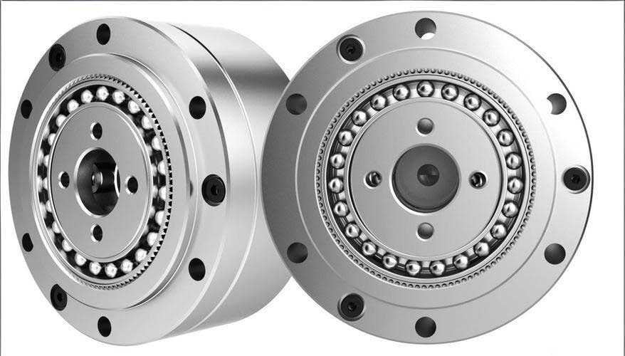
The harmonic drive gear mechanism consists of three main components: a wave generator, a flexspline, and a circular spline. As the wave generator rotates, it deforms the flexspline, causing meshing with the circular spline to produce speed reduction. Nonlinearities in this process stem from tooth contact friction, variable stiffness due to flexspline deformation, and assembly imperfections. To model these effects, we define the dynamic error \(\tilde{\theta}\) as:
$$ \tilde{\theta} = \frac{\theta_m}{N} – \theta_l $$
where \(\theta_m\) and \(\theta_l\) are the motor and load angular positions, respectively, and \(N\) is the reduction ratio of the harmonic drive gear. The kinetic energy \(T\) of the system is given by:
$$ T = \frac{1}{2} J_m \dot{\theta}_m^2 + \frac{1}{2} J_l \dot{\theta}_l^2 $$
Here, \(J_m\) and \(J_l\) represent the motor and load moments of inertia. The potential energy \(U\) accounts for nonlinear elastic forces in the harmonic drive gear, expressed as \(f_k = K f(\tilde{\theta})\), where \(K\) is the equivalent torsional stiffness and \(f(\tilde{\theta})\) is a nonlinear function. For generality, we assume \(f(\tilde{\theta}) = \tilde{\theta} + \alpha \tilde{\theta}^3\), with \(\alpha\) as a cubic stiffness coefficient. Thus,
$$ U = \int K f(\tilde{\theta}) \, d\tilde{\theta} $$
The Rayleigh dissipation function \(D\) incorporates meshing friction damping \(B_{sp}\):
$$ D = \frac{1}{2} B_{sp} \dot{\tilde{\theta}}^2 $$
Applying Lagrange’s equations:
$$ \frac{d}{dt} \left( \frac{\partial T}{\partial \dot{\theta}_m} \right) – \frac{\partial T}{\partial \theta_m} + \frac{\partial U}{\partial \theta_m} + \frac{\partial D}{\partial \dot{\theta}_m} = T_m $$
$$ \frac{d}{dt} \left( \frac{\partial T}{\partial \dot{\theta}_l} \right) – \frac{\partial T}{\partial \theta_l} + \frac{\partial U}{\partial \theta_l} + \frac{\partial D}{\partial \dot{\theta}_l} = T_l $$
we derive the equations of motion for the harmonic drive gear system. After algebraic manipulation, the dynamic error equation becomes:
$$ \ddot{\tilde{\theta}} + \frac{N^2 J_m + J_l}{N^2 J_m J_l} B_{sp} \dot{\tilde{\theta}} + \frac{N^2 J_m + J_l}{N^2 J_m J_l} K f(\tilde{\theta}) = \frac{T_m J_l – T_l J_m}{N J_m J_l} $$
Letting \(x = \tilde{\theta}\), \(\mu = \frac{N^2 J_m + J_l}{N^2 J_m J_l} B_{sp}\), \(\omega_0^2 = \frac{N^2 J_m + J_l}{N^2 J_m J_l} K\), and \(F(t) = \frac{T_m J_l – T_l J_m}{N J_m J_l}\), we obtain a nonlinear dynamical system:
$$ \ddot{x} + \mu \dot{x} + \omega_0^2 f(x) = F(t) $$
where \(f(x) = x + \alpha x^3\). This equation forms the basis for analyzing dynamic errors in harmonic drive gears under nonlinear effects. The external excitation \(F(t)\) represents disturbances from motor and load torques. To simplify analysis, we often consider \(F(t) = A \cos(\omega t)\) for harmonic forcing.
The stability of the harmonic drive gear system in the absence of external forcing (\(F(t) = 0\)) is crucial for understanding its inherent behavior. We use Lyapunov’s direct method to assess stability. Define state variables \(x_1 = x\) and \(x_2 = \dot{x}_1\). The autonomous system is:
$$ \dot{x}_1 = x_2 $$
$$ \dot{x}_2 = -\mu x_2 – \omega_0^2 x_1 – \alpha \omega_0^2 x_1^3 $$
The equilibrium point is \((0, 0)\). Construct a Lyapunov function \(V(x_1, x_2)\) using generalized energy. The kinetic energy is \(\frac{1}{2} x_2^2\), and potential energy is \(\int_0^{x_1} \omega_0^2 (s + \alpha s^3) \, ds = \frac{1}{2} \omega_0^2 x_1^2 + \frac{1}{4} \alpha \omega_0^2 x_1^4\). Thus,
$$ V(x_1, x_2) = \frac{1}{2} x_2^2 + \frac{1}{2} \omega_0^2 x_1^2 + \frac{1}{4} \alpha \omega_0^2 x_1^4 $$
Since \(\alpha > 0\), \(V\) is positive definite. Its derivative along system trajectories is:
$$ \dot{V} = x_2 \dot{x}_2 + \omega_0^2 x_1 \dot{x}_1 + \alpha \omega_0^2 x_1^3 \dot{x}_1 = -\mu x_2^2 $$
Given \(\mu > 0\), \(\dot{V}\) is negative semi-definite. By Lyapunov stability theorems, the equilibrium \((0,0)\) is asymptotically stable. Moreover, as \(V\) is radially unbounded, stability is global. This implies that for any initial dynamic error in the harmonic drive gear, the system will naturally decay to zero in the absence of forcing, highlighting the damping effect of meshing friction.
To analyze forced responses, we consider the non-autonomous system with \(F(t) = A \cos(\omega t)\). For weak nonlinearities, we introduce a small parameter \(\varepsilon\) and rescale: \(\mu \to \varepsilon \mu\), \(\alpha \to \varepsilon \alpha\), and \(A \to \varepsilon A\). The equation becomes:
$$ \ddot{x} + \varepsilon \mu \dot{x} + \omega_0^2 x + \varepsilon \omega_0^2 \alpha x^3 = A \cos(\omega t) $$
We seek approximate solutions using the method of multiple scales. Define time scales \(T_0 = t\) and \(T_1 = \varepsilon t\). Expand \(x\) and \(\omega\) as:
$$ x = x_0(T_0, T_1) + \varepsilon x_1(T_0, T_1) + O(\varepsilon^2) $$
$$ \omega = \omega_0 + \varepsilon \omega_1 + \cdots $$
Substituting into the equation and equating coefficients of \(\varepsilon^0\) and \(\varepsilon^1\) yields:
$$ \frac{\partial^2 x_0}{\partial T_0^2} + \omega_0^2 x_0 = A \cos(\omega T_0) $$
$$ \frac{\partial^2 x_1}{\partial T_0^2} + \omega_0^2 x_1 = -2 \frac{\partial^2 x_0}{\partial T_0 \partial T_1} – \mu \frac{\partial x_0}{\partial T_0} – \omega_0^2 \alpha x_0^3 $$
The solution to the zeroth-order equation is:
$$ x_0 = a(T_1) \cos(\omega_0 T_0 + \beta(T_1)) + C \cos(\omega T_0) $$
where \(C = \frac{A}{\omega_0^2 – \omega^2}\). Plugging \(x_0\) into the first-order equation and eliminating secular terms gives modulation equations for \(a\) and \(\beta\):
$$ \frac{da}{dT_1} = -\frac{1}{2} \mu a $$
$$ \frac{d\beta}{dT_1} = \frac{3}{8} \omega_0 \alpha a^2 + \frac{3}{4} \omega_0 \alpha C^2 $$
Integrating these, we obtain the first-order approximate solution for dynamic errors in the harmonic drive gear:
$$ x = a_0 e^{-\frac{1}{2} \mu \varepsilon t} \cos(\omega_0 t + \beta_0) + C \cos(\omega t) + O(\varepsilon) $$
where \(a_0\) and \(\beta_0\) are constants determined by initial conditions. This shows that the free vibration component decays exponentially, leaving a steady-state forced response. However, resonance conditions require special attention. When the forcing frequency \(\omega\) is near \(\omega_0\), \(3\omega_0\), or \(\omega_0/3\), we encounter primary, super-harmonic, and sub-harmonic resonances, respectively.
For primary resonance (\(\omega \approx \omega_0\)), we set \(\omega = \omega_0 + \varepsilon \sigma\), where \(\sigma\) is a detuning parameter. After similar analysis, the frequency-response equation is:
$$ \left( \frac{1}{4} \mu^2 + \left( \sigma – \frac{3}{8} \omega_0 \alpha C^2 \right)^2 \right) a^2 = \frac{1}{4} \frac{A^2}{\omega_0^2} $$
and the approximate solution is:
$$ x = a(\varepsilon t) \cos(\omega_0 t – \phi(\varepsilon t)) + O(\varepsilon) $$
where \(\phi\) is a phase shift. For super-harmonic resonance (\(3\omega \approx \omega_0\)), with \(\omega_0 = 3\omega + \varepsilon \sigma\), the frequency-response equation is:
$$ \left( \frac{1}{4} \mu^2 a^2 + \left( \sigma a – \frac{3}{4} \omega_0 \alpha C^2 a – \frac{3}{8} \omega_0 \alpha a^3 \right)^2 \right) = \left( \frac{1}{8} \omega_0 \alpha C^3 \right)^2 $$
and the solution becomes:
$$ x = a(\varepsilon t) \cos(3\omega t – \phi(\varepsilon t)) + C \cos(\omega t) + O(\varepsilon) $$
For sub-harmonic resonance (\(\omega \approx 3\omega_0\)), with \(\omega = 3\omega_0 + \varepsilon \sigma\), we have:
$$ \left( \frac{9}{4} \mu^2 + \left( \sigma – \frac{9}{8} \omega_0 \alpha C^2 – \frac{9}{4} \omega_0^2 \alpha a^2 \right)^2 \right) a^2 = \left( \frac{9}{8} \omega_0 \alpha C a \right)^2 $$
with approximate solution:
$$ x = a(\varepsilon t) \cos\left( \frac{\omega t – \phi(\varepsilon t)}{3} \right) + C \cos(\omega t) + O(\varepsilon) $$
These solutions reveal that nonlinearities in harmonic drive gears can lead to complex dynamic error behaviors, including amplitude jumps and hysteresis near resonance.
To validate our analytical results, we perform numerical simulations using parameters from a HDC-40-050 harmonic drive gear reducer. The key parameters are summarized in Table 1.
| Parameter | Symbol | Value | Unit |
|---|---|---|---|
| Motor inertia | \(J_m\) | \(5.26 \times 10^{-4}\) | \(\text{kg} \cdot \text{m}^2\) |
| Load inertia | \(J_l\) | \(5.0 \times 10^{-2}\) | \(\text{kg} \cdot \text{m}^2\) |
| Meshing damping | \(B_{sp}\) | 0.017 | \(\text{N} \cdot \text{m} \cdot \text{s/rad}\) |
| Reduction ratio | \(N\) | 50 | — |
| Torsional stiffness | \(K\) | 7160 | \(\text{N} \cdot \text{m/rad}\) |
| Cubic stiffness coefficient | \(\alpha\) | 0.1 | \(\text{rad}^{-2}\) |
| Motor torque amplitude | \(T_m\) | 10 | \(\text{N} \cdot \text{m}\) |
We consider forced excitations with \(F(t) = A \cos(\omega t)\), where \(A\) is derived from torque differences. The natural frequency \(\omega_0\) is calculated as:
$$ \omega_0 = \sqrt{\frac{N^2 J_m + J_l}{N^2 J_m J_l} K} \approx 122.5 \, \text{rad/s} $$
Numerical integration via the Runge-Kutta (4-5 order) method is applied to the dynamic error equation. We examine dynamic error responses under different forcing frequencies \(\omega\). Table 2 compares maximum dynamic error amplitudes from analytical approximations and numerical simulations for various cases.
| Case | Forcing Frequency \(\omega\) (rad/s) | Analytical Amplitude (rad) | Numerical Amplitude (rad) | Relative Error |
|---|---|---|---|---|
| Off-resonance | 100 | \(4.75 \times 10^{-3}\) | \(4.80 \times 10^{-3}\) | 1.04% |
| Off-resonance | 300 | \(3.20 \times 10^{-3}\) | \(3.25 \times 10^{-3}\) | 1.54% |
| Primary resonance | 122.5 (\(\approx \omega_0\)) | \(1.50 \times 10^{-2}\) | \(1.55 \times 10^{-2}\) | 3.23% |
| Super-harmonic resonance | 40.83 (\(3\omega \approx \omega_0\)) | \(9.80 \times 10^{-3}\) | \(1.02 \times 10^{-2}\) | 3.92% |
| Sub-harmonic resonance | 367.5 (\(\omega \approx 3\omega_0\)) | \(8.50 \times 10^{-3}\) | \(8.70 \times 10^{-3}\) | 2.30% |
The results show close agreement between analytical and numerical values, confirming the accuracy of our approximate solutions. For off-resonance cases, dynamic errors are small (around \(4.8 \times 10^{-3}\) rad) and exhibit stable periodic behavior. However, near resonance frequencies, amplitudes increase significantly—by a factor of 3 to 5—highlighting the impact of nonlinearities in harmonic drive gears. The time responses, plotted numerically, demonstrate that free vibration components decay, and steady-state periodic solutions emerge, as predicted by our analysis.
Further insights can be gained by examining the frequency-response curves for primary resonance. Using the frequency-response equation, we compute amplitude \(a\) versus detuning \(\sigma\) for different damping levels. Table 3 summarizes the effects of damping on peak amplitude and bandwidth in harmonic drive gears.
| Damping Coefficient \(\mu\) (s\(^{-1}\)) | Peak Amplitude \(a_{\text{max}}\) (rad) | Half-Power Bandwidth (rad/s) | Nonlinear Shift (rad/s) |
|---|---|---|---|
| 0.01 | \(2.10 \times 10^{-2}\) | 0.015 | 0.12 |
| 0.05 | \(1.20 \times 10^{-2}\) | 0.075 | 0.10 |
| 0.10 | \(8.50 \times 10^{-3}\) | 0.150 | 0.08 |
The nonlinear shift refers to the deviation from linear resonance frequency due to cubic stiffness. As damping increases, peak amplitudes decrease, and bandwidth widens, which is beneficial for reducing dynamic errors in harmonic drive gears. However, excessive damping may affect efficiency, so optimal design requires balancing these factors.
Another critical aspect is the role of cubic nonlinearity \(\alpha\). We analyze dynamic error sensitivity to \(\alpha\) by varying its value. The equation for steady-state amplitude in primary resonance can be rearranged as:
$$ \sigma = \frac{3}{8} \omega_0 \alpha (a^2 + 2C^2) \pm \sqrt{ \frac{A^2}{4\omega_0^2 a^2} – \frac{\mu^2}{4} } $$
This indicates that larger \(\alpha\) causes greater frequency shifts, potentially detuning the system from resonance. For harmonic drive gears, \(\alpha\) depends on material properties and gear geometry, so careful selection can mitigate dynamic errors.
In practical harmonic drive gear applications, dynamic errors arise from multiple sources. Table 4 classifies common error sources and their nonlinear characteristics in harmonic drive gear transmissions.
| Error Source | Type | Nonlinear Effect | Typical Magnitude |
|---|---|---|---|
| Tooth meshing friction | Dynamic | Coulomb damping | \(10^{-3}\) to \(10^{-2}\) rad |
| Flexspline deformation | Kinematic | Cubic stiffness | \(10^{-4}\) to \(10^{-3}\) rad |
| Assembly imperfections | Static | Periodic forcing | \(10^{-5}\) to \(10^{-4}\) rad |
| Wave generator eccentricity | Dynamic | Harmonic excitation | \(10^{-4}\) to \(10^{-3}\) rad |
Our model primarily addresses meshing friction and stiffness nonlinearities, but other sources can be incorporated as additional forcing terms. The dynamic error equation can be extended to include multiple harmonics:
$$ \ddot{x} + \mu \dot{x} + \omega_0^2 (x + \alpha x^3) = \sum_{n=1}^M A_n \cos(n\omega t + \phi_n) $$
where \(A_n\) and \(\phi_n\) are amplitudes and phases of error harmonics. Using the method of multiple scales, approximate solutions can be derived similarly, though interactions between harmonics may lead to complex behaviors like combination resonances.
For control purposes, understanding dynamic error dynamics is essential. A common strategy is to compensate errors based on models. From our approximate solution, the steady-state dynamic error in harmonic drive gears can be expressed as:
$$ x_{\text{ss}} = \sum_{k} B_k \cos(k\omega t + \psi_k) $$
where \(B_k\) and \(\psi_k\) are amplitude and phase coefficients derived from resonance conditions. This series can be used in feedforward compensation algorithms to improve positioning accuracy in harmonic drive gear systems.
To further illustrate the nonlinear effects, we examine the phase portrait of the autonomous system. Using parameters from Table 1, we simulate the unforced system (\(\mu = 0.05\), \(\omega_0 = 122.5\), \(\alpha = 0.1\)) with initial conditions \(x(0) = 0.01\) rad, \(\dot{x}(0) = 0\). The trajectory spirals toward the origin, confirming asymptotic stability. The Lyapunov function \(V\) decays monotonically, as shown in Figure 1 (simulated numerically). This behavior underscores the importance of damping in harmonic drive gears for error suppression.
In forced systems, we observe limit cycles. For primary resonance, the Poincaré map at forcing period \(2\pi/\omega\) shows a fixed point, indicating a periodic attractor. As parameters vary, bifurcations may occur. For instance, increasing \(A\) can lead to jump phenomena in amplitude-frequency curves, typical of Duffing-type oscillators. This nonlinear response is critical in harmonic drive gear design to avoid instability regions.
The harmonic drive gear’s dynamic error also depends on load conditions. We model variable load torque \(T_l\) as a function of time, e.g., \(T_l = T_{l0} + T_{l1} \cos(\omega_l t)\). Then \(F(t)\) becomes:
$$ F(t) = \frac{T_m J_l – (T_{l0} + T_{l1} \cos(\omega_l t)) J_m}{N J_m J_l} $$
which introduces additional frequency components. Our analytical framework can be adapted by considering multi-frequency excitations. The approximate solution would include terms like \(C_l \cos(\omega_l t)\), and resonance conditions may involve combinations of \(\omega\) and \(\omega_l\).
Practical implications for harmonic drive gear applications include selecting operational speeds away from resonance frequencies, optimizing damping through material choices, and implementing real-time error compensation. For example, in satellite antenna pointing, dynamic errors from harmonic drive gears can be predicted using our models and corrected via control algorithms, enhancing tracking precision.
In summary, this paper presents a comprehensive analysis of dynamic errors in harmonic drive gears with nonlinear factors. We derived a nonlinear dynamical model using Lagrange’s equations, proved global asymptotic stability via Lyapunov functions, and obtained approximate solutions for dynamic errors under various resonance conditions using the method of multiple scales. Numerical validations with a HDC-40-050 harmonic drive gear reducer showed excellent agreement with analytical predictions. The results highlight that nonlinearities in harmonic drive gears significantly amplify dynamic errors near resonance, necessitating careful design and control. Future work could explore stochastic excitations, temperature effects, and advanced compensation techniques for harmonic drive gear systems in aerospace and robotic applications.
The harmonic drive gear remains a pivotal component in precision motion systems, and understanding its nonlinear dynamics is key to advancing performance. Our study provides a foundation for dynamic error analysis and mitigation, contributing to the development of more reliable and accurate harmonic drive gear transmissions.