
In the field of mechanical transmission systems, achieving smooth, efficient, and quiet operation is a perpetual engineering challenge. Among various gear configurations, the worm-helical gear pair stands out as a unique and valuable solution for applications requiring compact, high-ratio power transmission between non-parallel, non-intersecting shafts. This system consists of an involute cylindrical worm meshing with an involute helical gear, forming a point-contact engagement. While offering significant advantages such as a large reduction ratio, design flexibility, and relatively low manufacturing cost, its dynamic behavior is inherently complex. The core of this complexity, and the primary source of vibration and noise, lies in the internal excitations generated within the mesh. As an engineer specializing in gear dynamics, I find that mastering these excitations—primarily the time-varying mesh stiffness (TVMS) and the nonlinearities induced by factors like backlash and transmission errors—is absolutely essential for designing high-performance, reliable worm-helical gear drives. This article provides a detailed, first-person perspective on modeling the TVMS for this specific gear pair and analyzing its profound implications on the system’s nonlinear dynamic characteristics.
The fundamental operating principle of a worm-helical gear pair is based on the engagement between a screw-like worm and a helical gear whose teeth are cut at an angle. Unlike parallel-axis spur or helical gears with line contact, the theoretical contact between these two members is a point, which elongates into an elliptical contact patch under load. This point-contact characteristic inherently affects the load distribution, stiffness, and lubrication regime. Helical gears are chosen for their smoother engagement compared to spur gears, as the angled teeth allow for gradual load transfer, reducing impact noise. The combination with a worm allows for a very high speed reduction in a single stage. Understanding the dynamic performance requires us to first dissect and accurately model its most critical internal excitation: the time-varying mesh stiffness.
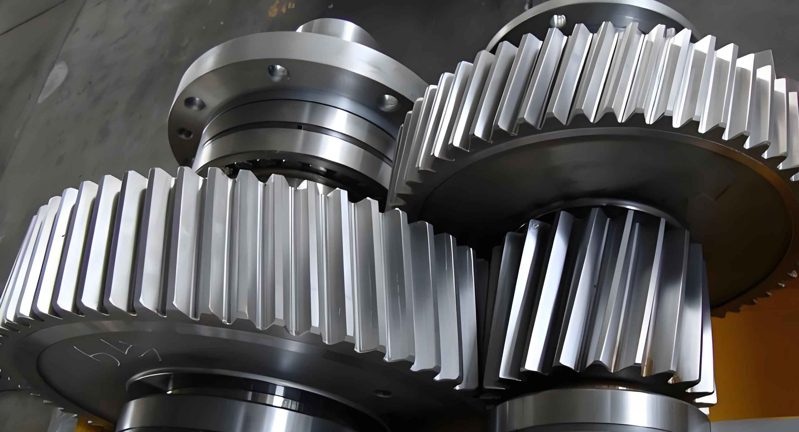
Modeling Time-Varying Mesh Stiffness for Worm-Helical Gear Pairs
The mesh stiffness of a gear pair is defined as the ratio of the meshing force to the total elastic deformation of the mating teeth along the line of action. It is not constant but varies periodically as the number of tooth pairs in contact changes and as the contact position moves along the tooth profile. For standard spur gears, this results in a characteristic rectangular waveform. For worm-helical gears, the situation is more intricate due to the point contact and the inclined contact line across the face width. The total deformation of a tooth under load comprises several components: Hertzian contact deformation, bending deflection, shear deformation, axial compressive deformation, and deformation of the gear body (fillet foundation). The total effective mesh stiffness is therefore the combined effect of these compliant elements acting in series for each contacting tooth pair.
To calculate this, I employ and adapt the potential energy method. This method models each tooth as a non-uniform cantilever beam fixed at the root circle (a more accurate boundary than the base circle). The stiffness contributions are derived from the strain energies associated with each deformation type. The key adaptation for worm-helical gears lies in treating the contact. Instead of a line of contact with a constant length, we consider a discretized series of contact points across the face width, each with an instantaneous elliptical contact area. The effective stiffness contribution at each slice is then summed.
The Hertzian contact stiffness, representing the local contact deformation, is given by:
$$k_h = \frac{L}{8\left(\frac{1-\nu_1^2}{\pi E_1} + \frac{1-\nu_2^2}{\pi E_2}\right)}$$
where \(L\) is related to the semi-major axis of the contact ellipse at the specific mesh position, and \(\nu_i\), \(E_i\) are the Poisson’s ratios and Young’s moduli of the worm and gear materials, respectively.
The bending, shear, and axial compressive stiffnesses for a slice of the helical gear tooth are calculated via integral expressions along the tooth profile from the root to the contact point. For bending:
$$k_b^{-1} = \int_{\alpha_1}^{\alpha_2} \frac{3\{1+\cos\alpha_1[(\alpha_2-\alpha)\sin\alpha – \cos\alpha]\}^2 (\alpha_2-\alpha)\cos\alpha}{2E [\sin\alpha + (\alpha_2-\alpha)\cos\alpha]^3 \Delta b} d\alpha + \text{(Root contribution)}$$
where \(\alpha\) is the pressure angle variable, \(\alpha_1, \alpha_2\) are angles related to the contact point and base circle, and \(\Delta b\) is the projection of the contact ellipse dimension. Similar integral expressions define the shear stiffness \(k_s\) and axial compressive stiffness \(k_a\).
The fillet foundation stiffness \(k_f\) accounts for the compliance of the gear body below the tooth and is often calculated using empirical formulas based on gear geometry parameters.
For a single pair of teeth in contact, the combined mesh stiffness \(k_{pair}\) is:
$$k_{pair} = \left( \frac{1}{k_{h}} + \frac{1}{k_{b,w}+k_{s,w}+k_{a,w}+k_{f,w}} + \frac{1}{k_{b,g}+k_{s,g}+k_{a,g}+k_{f,g}} \right)^{-1}$$
where subscripts \(w\) and \(g\) denote worm and gear contributions. For worm-helical gears, the axial stiffness of the worm thread can be significant and must be carefully included.
When the total contact ratio is between 1 and 2, the gear pair undergoes alternating single and double-tooth contact. The total mesh stiffness \(k(t)\) is the sum of the stiffnesses of all concurrent contacting pairs:
$$k(t) = \sum_{j=1}^{N_p} k_{pair, j}(t)$$
where \(N_p\) is the number of tooth pairs in contact (1 or 2). This summation yields a periodic, time-varying stiffness function. For dynamic analysis, this periodic function can be approximated by its average value plus a harmonic variation:
$$k(t) = k_m + k_a \cos(\omega_m t + \phi)$$
where \(k_m\) is the average mesh stiffness, \(k_a\) is the stiffness variation amplitude, \(\omega_m\) is the gear mesh frequency, and \(\phi\) is a phase angle.
The following table summarizes the different stiffness components and their primary influencing factors for worm-helical gears:
| Stiffness Component | Physical Origin | Key Influencing Factors (Worm-Helical Gear Specific) |
|---|---|---|
| Hertzian Contact Stiffness (\(k_h\)) | Local deformation of surfaces at the contact point/ellipse. | Material properties (E, ν), curvature radii at contact, contact ellipse dimensions (function of helix angles and alignment). |
| Bending Stiffness (\(k_b\)) | Deflection of tooth as a cantilever beam under bending moment. | Tooth geometry (module, pressure angle, profile), face width, contact point position, helix angle affecting effective cantilever length. |
| Shear Stiffness (\(k_s\)) | Deflection due to shear forces. | Tooth cross-sectional area, shear modulus, contact position. |
| Axial Compressive Stiffness (\(k_a\)) | Shortening of tooth due to axial component of mesh force. | Helix angle (critical for both worm and helical gear), tooth cross-section. |
| Fillet Foundation Stiffness (\(k_f\)) | Deformation of gear body supporting the tooth root. | Rim thickness, hub geometry, number of teeth. |
Nonlinear Dynamic Modeling of the Transmission System
With a reliable model for the TVMS in place, the next step is to investigate how this excitation, coupled with other real-world factors, influences the system’s dynamic response. To do this, I develop a lumped-parameter torsional vibration model. The system is reduced to two degrees of freedom: the rotational displacements of the worm (\(\theta_w\)) and the helical gear (\(\theta_g\)). The model incorporates the three most significant sources of nonlinearity and excitation in gear dynamics: the time-varying mesh stiffness \(k(t)\), the static transmission error \(e(t)\) (representing composite manufacturing and alignment errors), and the gear backlash \(2b\).
The equations of motion derived from force and torque balances are:
$$J_w \ddot{\theta}_w + c_n r_{bw}\cos\beta_w [ r_{bw}\dot{\theta}_w – r_{bg}\dot{\theta}_g – \dot{e}(t)] + k(t) r_{bw}\cos\beta_w \cdot f(r_{bw}\theta_w – r_{bg}\theta_g – e(t)) = T_w$$
$$J_g \ddot{\theta}_g – c_n r_{bg}\cos\beta_g [ r_{bw}\dot{\theta}_w – r_{bg}\dot{\theta}_g – \dot{e}(t)] – k(t) r_{bg}\cos\beta_g \cdot f(r_{bw}\theta_w – r_{bg}\theta_g – e(t)) = -T_g$$
where \(J\), \(r_b\), \(\beta\), and \(T\) denote mass moment of inertia, base circle radius, helix angle, and torque, respectively. \(c_n\) is the linear mesh damping. The function \(f(x)\) is the backlash nonlinearity function, defined as:
$$f(x) = \begin{cases} x – b, & x > b \\ 0, & |x| \le b \\ x + b, & x < -b \end{cases}$$
This piecewise function is responsible for the system’s most severe nonlinear behavior, including tooth separation and impacts upon re-engagement.
To analyze the system effectively, it’s standard practice to reduce the two equations to a single equation describing the dynamic transmission error along the line of action, defined as \(x(t) = r_{bw}\theta_w – r_{bg}\theta_g – e(t)\). Furthermore, we non-dimensionalize the equation to improve numerical conditioning and generalize the results. Introducing non-dimensional time \(\tau = \omega_n t\), where \(\omega_n = \sqrt{k_m/m_e}\) is the natural frequency, and non-dimensional displacement \(\bar{x} = x/b\), we obtain:
$$f_n + f_e \omega^2 \cos\tau = \ddot{\bar{x}} + 2\zeta(\cos\beta_w + \cos\beta_g)\dot{\bar{x}} + (\cos\beta_w + \cos\beta_g)[1 + k_1\cos(\tau)]f[\bar{x}(\tau)]$$
Here, \(m_e\) is the equivalent mass, \(\zeta\) is the damping ratio, \(f_n\) is the normalized static force, \(f_e\) is the normalized error amplitude (\(e_0/b\)), \(\omega\) is the frequency ratio (\(\omega_m/\omega_n\)), and \(k_1\) is the normalized stiffness variation amplitude (\(k_a/k_m\)). The function \(f[\bar{x}]\) is the non-dimensional backlash function with a unity threshold.
Analysis of Dynamic Response and Parametric Influences
Solving the non-dimensional nonlinear differential equation requires numerical integration. I typically use a variable-step 4th-5th order Runge-Kutta method (like MATLAB’s ode45), discarding an initial transient to obtain the steady-state dynamic response. The system’s behavior is then analyzed using a suite of tools: time-domain waveforms, phase portraits, Poincaré maps (sampling the state at the mesh period), and Fast Fourier Transform (FFT) spectra. By varying key system parameters, we can map out the rich and complex dynamic landscape of the worm-helical gear system.
Influence of Backlash (\(b\))
Backlash is an essential clearance to prevent jamming and allow for lubrication, but it introduces severe nonlinearity. My analysis shows that while the absolute amplitude of vibration increases with larger backlash, the fundamental nature of the dynamic state for lightly loaded systems often remains a stable period-1 or quasi-periodic motion. The backlash primarily governs the severity of impacts when teeth re-engage after separation. A Poincaré map for a system with moderate backlash typically shows a concentrated cluster of points, indicating a steady, predictable motion. However, for a fixed error, increasing backlash effectively reduces the normalized force parameter \(f_n\), which can push the system towards chaotic regimes.
Influence of Load / Static Force (\(f_n\) via Error \(f_e\))
The load condition, often encapsulated in the ratio \(f_n/f_e\), is a critical driver of dynamic state changes. For a constant input torque, varying the amplitude of the static transmission error \(f_e\) simulates the effect of different manufacturing precision levels or misalignments. My parametric studies reveal distinct dynamic regimes:
| Error Amplitude Range (\(f_e\)) | Typical Dynamic State | Characteristics |
|---|---|---|
| Very Small (e.g., < 0.06) | Periodic (P-1) or Quasi-Periodic Motion | Stable, low vibration. Poincaré map shows a finite set of points or a closed curve. |
| Moderate (e.g., 0.06 – 0.15) | Chaotic Motion | Aperiodic, sensitive to initial conditions. Poincaré map shows a scattered, fractal-like structure. Broadband FFT spectrum. |
| Large (e.g., > 0.15) | High-periodic or Chaotic Motion | Possibly reverting to periodic motion at very high error levels, but with severe impacts and large amplitude. |
This demonstrates that to ensure stable, low-vibration operation of worm-helical gear drives, controlling manufacturing and assembly errors (minimizing \(f_e\)) is as crucial as proper stiffness design.
Influence of Speed / Frequency Ratio (\(\omega\))
Varying the input speed changes the meshing frequency and thus the frequency ratio \(\omega\). This is analogous to conducting a “frequency sweep” on the nonlinear system. The resulting bifurcation diagram, plotting the dynamic transmission error against speed, is highly complex. For worm-helical gears, I observe that the system is often in a chaotic state across wide speed ranges. However, there exist “islands” of stability—specific speed ranges where the motion becomes periodic or quasi-periodic. For instance, within a certain mid-range speed band (e.g., corresponding to \(\omega\) near certain sub-harmonics of the natural frequency), the system may exhibit period-2, period-4, or other higher-order periodic motions. The Poincaré map in these stable islands shows a precise number of discrete points. This finding is critical for designers: it implies that for a given design, there may be optimal operating speeds that inherently promote smoother running and lower noise.
Influence of Damping Ratio (\(\zeta\))
Damping, arising from material hysteresis, lubrication, and bearings, is a stabilizing factor. My simulations consistently show that increasing the damping ratio \(\zeta\) suppresses chaotic behavior and narrows the regions of instability in parameter space. Higher damping attenuates the severity of impacts caused by the backlash nonlinearity and reduces the amplification of vibrations near resonance conditions. For worm-helical gear systems, especially those with polymer gears where material damping can be significant, this effect can be a key advantage in achieving smooth operation even in the presence of other excitations.
The interplay of these parameters can be summarized for design guidance:
| Design / Operational Parameter | Effect on Dynamic Stability | Practical Design Implication |
|---|---|---|
| Reduce Backlash (\(b\)) | Reduces impact severity and nonlinear jump phenomena; may not alter fundamental state if small. | Minimize to functional minimum; use anti-backlash designs if critical. |
| Reduce Error (\(f_e\)) | Strongly promotes periodic, stable motion; pushes system away from chaos. | Invest in high-precision manufacturing and robust alignment procedures for the worm and helical gear. |
| Optimize Operating Speed (\(\omega\)) | Can move system from chaotic zones into stable periodic “islands”. | Conduct dynamic analysis to identify and target stable speed ranges for the application. |
| Increase Damping (\(\zeta\)) | Suppresses vibration amplitudes and stabilizes the response across parameter ranges. | Consider gear materials with higher inherent damping (e.g., polymers), optimized lubricants, and integrated damping elements. |
Discussion and Design Implications
The analysis clearly demonstrates that the dynamics of worm-helical gear systems are governed by a delicate balance between internal excitations and system parameters. The time-varying mesh stiffness acts as a fundamental parametric exciter. When its variation frequency and harmonics interact with the system’s nonlinear resonances (governed by backlash and modulated by error), complex dynamic states like quasi-periodicity and chaos can emerge. These states are characterized by increased vibration levels, elevated noise, and potentially higher dynamic loads that accelerate wear and fatigue.
The practical significance of these findings is substantial. For engineers designing such transmissions for applications in automotive systems, robotics, or precision instruments, the goal is to avoid chaotic and high-impact regimes. The models and results presented here provide a roadmap:
- Stiffness Design: While the TVMS cannot be eliminated, its amplitude \(k_a\) can be influenced. Optimizing tooth geometry for helical gears (e.g., pressure angle, helix angle, addendum modification) can help maximize the average stiffness \(k_m\) while potentially smoothing the transition between single and double tooth contact, reducing the stiffness variation.
- Error and Backlash Control: This is paramount. Tight tolerances for the worm and helical gear, along with precise housing and bearing alignment to minimize static transmission error, are the most effective ways to promote stable dynamics. Backlash should be controlled to the minimum functional value.
- System Tuning: Understanding the bifurcation behavior with speed allows designers to specify “quiet zones” for operation or to add speed-varying controls (like inverters) to avoid problematic resonant speeds.
- Damping Utilization: The beneficial role of damping should be leveraged. In systems with steel worms and polymer helical gears, the polymer’s damping can be a significant asset for vibration suppression, making this material combination dynamically favorable despite lower stiffness.
In conclusion, the path to low-vibration, low-noise worm-helical gear transmissions lies in a holistic design approach that integrates accurate modeling of the unique point-contact TVMS with a thorough nonlinear dynamic analysis. By treating the gear pair not just as a static torque transmitter but as a dynamic system responsive to stiffness, error, and clearance, we can make informed decisions on geometry, tolerances, materials, and operating conditions. This empowers us to push these compact, high-ratio drives into more demanding applications where performance and reliability are critical, ultimately extending their service life and expanding their utility in modern machinery. The continued exploration of these dynamics, including effects of thermal changes, wear evolution, and more advanced contact models, remains a vital and rewarding area of research and engineering development.