
In modern automotive engineering, particularly with the continuous increase in vehicle speed and demand for power density, the hypoid gear set serving as the primary reducer in the drive axle is subjected to increasingly severe operational conditions. These conditions push the gears to very high rotational speeds, making the analysis of dynamic loads, vibration, noise, and potential failure modes a critical concern for reliability and NVH (Noise, Vibration, and Harshness) performance. The vibration excitation in gear systems arises from several intrinsic factors, including time-varying mesh stiffness, static transmission error, and the unavoidable presence of backlash. While backlash is essential for providing adequate lubrication and preventing tooth interference, its presence introduces strong nonlinearity into the system dynamics. This nonlinearity can lead to phenomena such as tooth separation, re-engagement impacts, complex subharmonic and chaotic motions, which significantly amplify dynamic loads, exacerbate noise, and ultimately compromise the fatigue life and reliability of the gear transmission. While substantial research has been conducted on the nonlinear dynamics of parallel-axis spur and helical gears, the complex spatial geometry of hypoid gears has presented significant challenges, leaving a notable gap in the literature regarding their detailed nonlinear vibration analysis. This article aims to address this gap by establishing and solving a nonlinear dynamic model tailored for hypoid gear pairs.
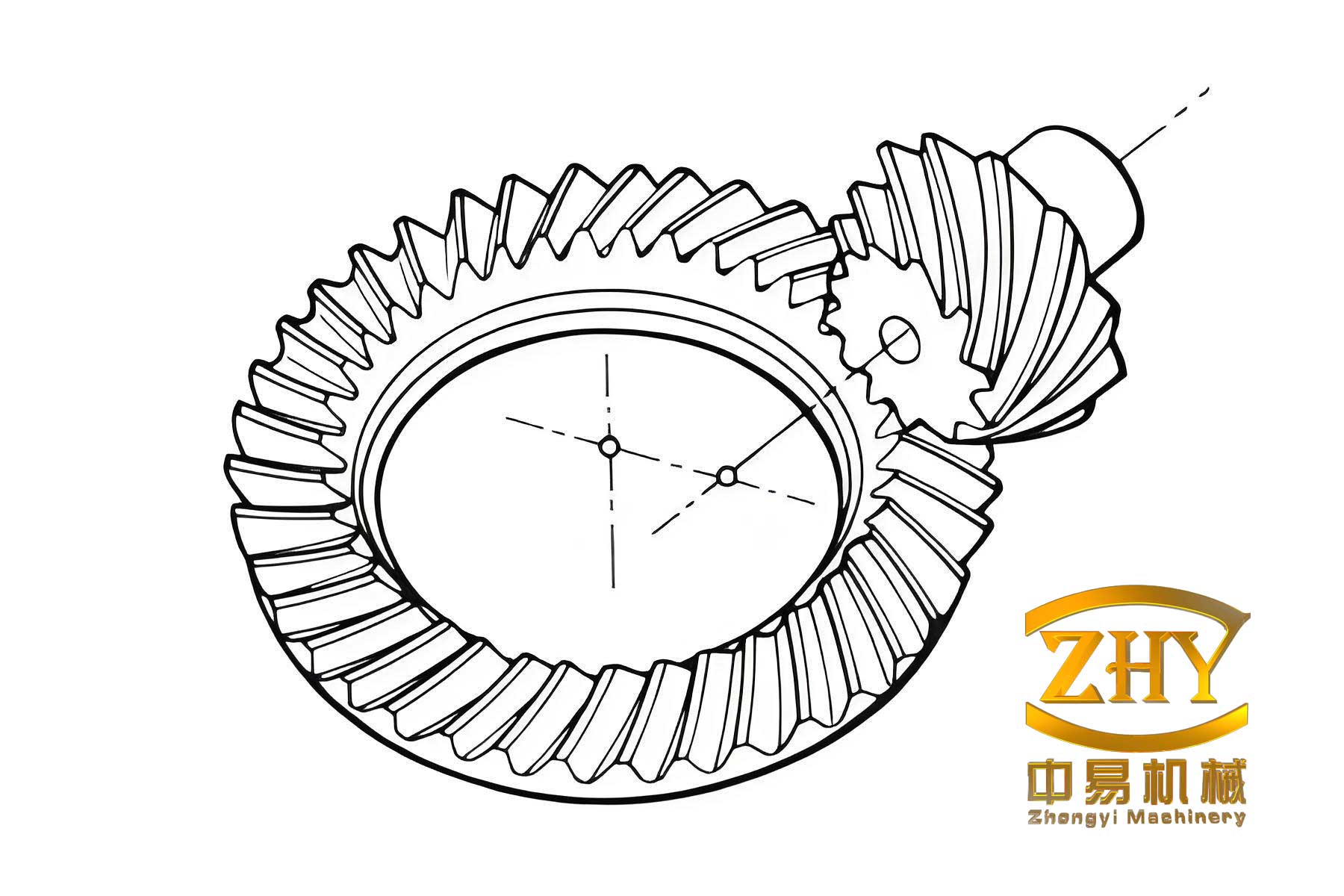
The core of this analysis is the development of a simplified yet physically representative nonlinear vibration model for a hypoid gear pair. The model condenses the system to a single degree of freedom (SDOF) by considering the torsional vibrations of the pinion and gear, lumped with their respective input and output inertias assuming rigid shafts. The governing equation incorporates the three key excitations: periodic fluctuation of the mesh stiffness \( k(t) \), the static transmission error excitation \( e(t) \), and a piecewise-linear backlash function \( f_b(x) \). The dynamic transmission error (DTE) along the line of action is chosen as the primary coordinate. The figure below illustrates a typical hypoid gear set, highlighting the offset between axes that defines its geometry and influences its contact and dynamic behavior.
The derivation begins with the equations of motion for the pinion and gear. Considering moments about their rotation axes and projecting forces onto the normal direction of the mesh, we obtain:
$$ I_p \ddot{\theta}_p = T_p – R_{bp} [c(\dot{x} – \dot{e}) + k(t)f_b(x – e)] $$
$$ I_g \ddot{\theta}_g = -T_g + R_{bg} [c(\dot{x} – \dot{e}) + k(t)f_b(x – e)] $$
where \( I_p, I_g \) are the mass moments of inertia, \( \theta_p, \theta_g \) are angular displacements, \( T_p, T_g \) are input and output torques, \( R_{bp}, R_{bg} \) are base circle radii (or their effective equivalents for hypoid gears), \( c \) is the mesh damping coefficient, and \( x \) is the relative dynamic displacement along the line of action. The term \( f_b(x – e) \) represents the nonlinear displacement function due to backlash. Defining the dynamic transmission error \( \delta = x – e \), and combining the two equations to eliminate the internal force, we arrive at a single equation:
$$ m_{eq} \ddot{\delta} + c \dot{\delta} + k(t) f_b(\delta) = F_{m} – m_{eq} \ddot{e}(t) $$
Here, \( m_{eq} = 1 / ( (R_{bp})^2/I_p + (R_{bg})^2/I_g ) \) is the equivalent mass, and \( F_m = T_p / R_{bp} = T_g / R_{bg} \) is the average static mesh force. The backlash function \( f_b(\delta) \) is classically defined as a piecewise-linear function:
$$ f_b(\delta) =
\begin{cases}
\delta – b, & \delta > b \\
0, & -b \le \delta \le b \\
\delta + b, & \delta < -b
\end{cases} $$
where \( 2b \) is the total gear backlash. The time-varying mesh stiffness \( k(t) \) and static transmission error \( e(t) \) are periodic functions with the mesh frequency \( \omega_m = Z_p \Omega_p = Z_g \Omega_g \), where \( Z \) and \( \Omega \) denote tooth count and rotational speed. They can be represented by Fourier series:
$$ k(t) = k_0 + \sum_{n=1}^{N} k_n \cos(n\omega_m t + \phi_n^k) $$
$$ e(t) = \sum_{n=1}^{M} e_n \cos(n\omega_m t + \phi_n^e) $$
To generalize the analysis, we introduce non-dimensional parameters. Let \( \omega_n = \sqrt{k_0 / m_{eq}} \) be the natural frequency based on the mean stiffness, \( \tau = \omega_n t \) be non-dimensional time, and \( X = \delta / b_c \) be non-dimensional displacement where \( b_c \) is a characteristic length (often related to \( b \) or \( e_n \)). The damping ratio is \( \zeta = c / (2 m_{eq} \omega_n) \). After manipulation, the non-dimensional equation of motion becomes:
$$ X” + 2\zeta X’ + \kappa(\tau) \cdot \text{fb}(X) = \bar{F}_m + \bar{E}(\tau) $$
where \( \kappa(\tau) = k(\tau)/k_0 \), \( \text{fb}(X) \) is the non-dimensional backlash function, \( \bar{F}_m \) is related to the static load, and \( \bar{E}(\tau) \) encapsulates the inertial excitation from \( e(t) \). This strong nonlinear, parametrically and externally excited differential equation forms the basis for the dynamic analysis of the hypoid gear system.
The numerical solution of this type of nonlinear periodic system is non-trivial, requiring robust algorithms beyond simple time-step integration for generating frequency response curves. The shooting method, combined with parameter continuation and arc-length parameterization, provides a powerful framework. First, the second-order non-dimensional equation is converted into a state-space form:
$$ \mathbf{y}’ = \mathbf{f}(\tau, \mathbf{y}, \lambda), \quad \mathbf{y} = [X, X’]^T $$
where \( \lambda \) represents a system parameter, typically the excitation frequency ratio \( \bar{\omega} = \omega_m / \omega_n \). For a periodic solution with period \( T = 2\pi/\bar{\omega} \), the boundary condition is \( \mathbf{y}(T) – \mathbf{y}(0) = \mathbf{0} \). The shooting method treats this as a root-finding problem: find initial conditions \( \mathbf{y}(0) = \mathbf{s} \) such that the defect \( \mathbf{G}(\mathbf{s}, \lambda) = \mathbf{y}(T; \mathbf{s}) – \mathbf{s} = \mathbf{0} \). Newton-Raphson iteration is used:
$$ \mathbf{s}^{(j+1)} = \mathbf{s}^{(j)} – \left[ \frac{\partial \mathbf{G}}{\partial \mathbf{s}} \right]^{-1} \mathbf{G}(\mathbf{s}^{(j)}, \lambda) $$
The crucial component is the Jacobian \( \partial \mathbf{G}/\partial \mathbf{s} = \mathbf{\Phi}(T) – \mathbf{I} \), where \( \mathbf{\Phi}(T) \) is the state transition matrix. This matrix is obtained by simultaneously integrating the original state equations and the variational equations \( \mathbf{\Phi}’ = \mathbf{J}(\tau) \mathbf{\Phi} \), with \( \mathbf{\Phi}(0)=\mathbf{I} \) and \( \mathbf{J}(\tau) = \partial \mathbf{f}/\partial \mathbf{y} \).
To trace solution branches (frequency response curves), a continuation method is employed. After finding a solution \( (\mathbf{s}_0, \lambda_0) \), we predict the next solution for \( \lambda_1 = \lambda_0 + \Delta \lambda \) by computing the tangent vector \( [d\mathbf{s}/d\lambda, 1]^T \) from:
$$ \frac{\partial \mathbf{G}}{\partial \mathbf{s}} \frac{d\mathbf{s}}{d\lambda} + \frac{\partial \mathbf{G}}{\partial \lambda} = \mathbf{0} $$
and then use \( \mathbf{s}_1^{pred} = \mathbf{s}_0 + (d\mathbf{s}/d\lambda) \Delta \lambda \). This predictor is corrected using the shooting method. This standard continuation fails at turning points (folds) where \( \partial \mathbf{G}/\partial \mathbf{s} \) becomes singular. To handle this, arc-length continuation is used, where the solution parameter becomes the arc-length \( \eta \) itself. The system is augmented with the pseudo-arclength condition:
$$ \mathbf{N}(\mathbf{s}, \lambda, \eta) \equiv \left( \frac{d\mathbf{s}}{d\eta} \right)^T (\mathbf{s} – \mathbf{s}_0) + \frac{d\lambda}{d\eta} (\lambda – \lambda_0) – \Delta \eta = 0 $$
We now solve the enlarged system \( \mathbf{H}(\mathbf{s}, \lambda) = [\mathbf{G}(\mathbf{s}, \lambda), N(\mathbf{s}, \lambda)]^T = \mathbf{0} \) for \( (\mathbf{s}, \lambda) \) as \( \eta \) varies. The Jacobian of this system is non-singular at turning points, allowing the path to be followed smoothly. Bifurcation points, where solution stability changes, can be detected by monitoring the eigenvalues of the monodromy matrix \( \mathbf{\Phi}(T) \); a pair crossing the unit circle indicates a Hopf bifurcation, while an eigenvalue crossing +1 often indicates a saddle-node or pitchfork bifurcation.
A summary of the key parameters used in a representative simulation of a hypoid gear nonlinear vibration analysis is provided in the table below. These parameters, including inertia, stiffness, error amplitudes, and damping, are crucial for defining the system’s dynamic character.
| Parameter | Symbol | Value | Unit |
|---|---|---|---|
| Equivalent Mass | \( m_{eq} \) | 0.05 | kg |
| Mean Mesh Stiffness | \( k_0 \) | 2.5e8 | N/m |
| Stiffness Variation Amplitude | \( \Delta k / k_0 \) | 0.2 | – |
| Fundamental STE Amplitude | \( e_1 \) | 10 | μm |
| Second Harmonic STE Amplitude | \( e_2 \) | 2 | μm |
| Backlash (Half) | \( b \) | 20 | μm |
| Mesh Damping Ratio | \( \zeta \) | 0.05 | – |
| Pinion Teeth | \( Z_p \) | 11 | – |
| Gear Teeth | \( Z_g \) | 41 | – |
| Mean Load (Non-dim.) | \( \bar{F}_m \) | 0.3 | – |
Applying the numerical methods described, the frequency response of the hypoid gear system can be computed. The primary resonance near \( \bar{\omega} = 1 \) exhibits the classic bending and hysteresis jump phenomena due to the nonlinear backlash. The amplitude of the non-dimensional dynamic transmission error \( |X| \) is plotted against the excitation frequency ratio. The following observations are critical:
- Primary Resonance Region: The response curve bends to the right, indicating a hardening-type nonlinearity induced by the loss of contact. As frequency is swept up, the amplitude jumps down at a point; when swept down, it jumps up at a different point, creating a hysteresis loop.
- Multi-Stability: Within the hysteresis region, three periodic solutions coexist: two stable (high-amplitude and low-amplitude) and one unstable saddle solution. The initial conditions determine which stable attractor the system settles into.
- Subharmonic and Chaotic Response: For higher forcing levels or specific parameter combinations, the analysis may reveal regions of period-2, period-4, or even chaotic motion, characterized by a broad spectrum and sensitive dependence on initial conditions.
- Influence of Hypoid Gear Parameters: The specific geometry of the hypoid gear influences the phase and amplitude of the higher harmonics in \( k(t) \) and \( e(t) \), which can excite super-harmonic resonances (e.g., near \( \bar{\omega} = 0.5, 0.33 \)) or modulate the primary resonance shape.
The dynamic response is highly sensitive to operational parameters. The table below summarizes the effect of varying key parameters on the resonance behavior of the hypoid gear system.
| Parameter Variation | Effect on Primary Resonance Peak | Effect on Backlash-Induced Jumps | Notes on Hypoid Gear Specifics |
|---|---|---|---|
| Increased Mean Load (\( \bar{F}_m \uparrow \)) | Amplitude decreases, peak shifts slightly right | Hysteresis region narrows; system spends less time in lost contact | Higher torque in hypoid gears increases contact ratio and can smooth stiffness variation. |
| Increased Backlash (\( b \uparrow \)) | Amplitude increases significantly, peak shifts right | Hysteresis region widens; severity of impacts increases | Backlash control is critical in hypoid gear assembly to manage dynamics and noise. |
| Increased STE Amplitude (\( e_1 \uparrow \)) | Amplitude increases, can excite stronger super-harmonics | Can initiate tooth separation at lower loads, affecting jump points | Hypoid gear surface topography and alignment errors directly affect \( e(t) \). |
| Increased Stiffness Variation (\( \Delta k / k_0 \uparrow \)) | Parametric excitation effects grow; may lead to instability regions | Can interact with backlash to create complex modulation | The varying contact path in hypoid gears results in a unique \( k(t) \) waveform. |
| Increased Damping (\( \zeta \uparrow \)) | Amplitude reduces sharply, peak broadens | Hysteresis region narrows; jump discontinuities become smoother | Mesh damping in hypoid gears is influenced by lubricant and tooth geometry. |
The implications of this nonlinear analysis for the design and operation of hypoid gears in automotive axles are profound. First, the prediction of dynamic load factors is essential for fatigue life calculation. The maximum dynamic mesh force \( F_{dyn} = k(t) f_b(\delta) \) can be significantly higher than the static load, especially during resonant conditions or during traversal of jump discontinuities. Second, radiated noise is closely correlated with the acceleration levels of the gear bodies, which are directly obtained from the second derivative of the dynamic transmission error \( \ddot{\delta} \). The analysis helps identify “critical speeds” or frequency ranges where noise and vibration are amplified. Third, understanding the multi-stable regions is crucial for startup/shutdown transient analysis and for diagnosing unexpected vibrations. A system operating in the high-amplitude branch of the hysteresis loop will have vastly different performance characteristics than one operating in the low-amplitude branch, even at the same nominal speed and load.
In conclusion, this work establishes a foundational framework for the nonlinear vibration analysis of hypoid gear pairs. By developing a single-degree-of-freedom model that incorporates the essential nonlinearities of time-varying mesh stiffness, static transmission error, and backlash, and by implementing advanced numerical solution techniques like the shooting method with arc-length continuation, we can effectively predict the complex dynamic behavior of these critical automotive components. The resulting frequency response curves reveal characteristic nonlinear phenomena such as resonance bending, hysteresis, and jump discontinuities, which are vital for assessing dynamic loads, noise potential, and operational stability. While the model presented is for hypoid gears, its mathematical structure is general and can be adapted, with appropriate modifications to the excitation functions \( k(t) \) and \( e(t) \), to analyze other gear types such as helical or spiral bevel gears. Future work should focus on extending this model to multiple degrees of freedom to include shaft flexibilities and bearing dynamics, incorporating more realistic friction models at the mesh, and validating the predictions against extensive experimental measurements from hypoid gear test rigs and actual automotive axle assemblies. Ultimately, this analytical capability will contribute to the design of quieter, more durable, and higher-performance hypoid gear drives for next-generation vehicles.