
I present a numerical-calculation-based methodology for controlling the tooth profile accuracy of a straight bevel gear produced by near-net shaping. The method is motivated by a practical difficulty: plastic forming can create a complete straight bevel gear tooth profile without machining, but the final geometry is affected by elastic recovery, die elasticity, contact modification, friction, and non-uniform deformation. If these effects are ignored, the resulting straight bevel gear may have acceptable macro-geometry but poor meshing behavior, excessive transmission error, and a contact pattern that is not robust under load. I therefore treat the forming die cavity as a geometry that must be corrected numerically rather than simply copied from the theoretical straight bevel gear model.
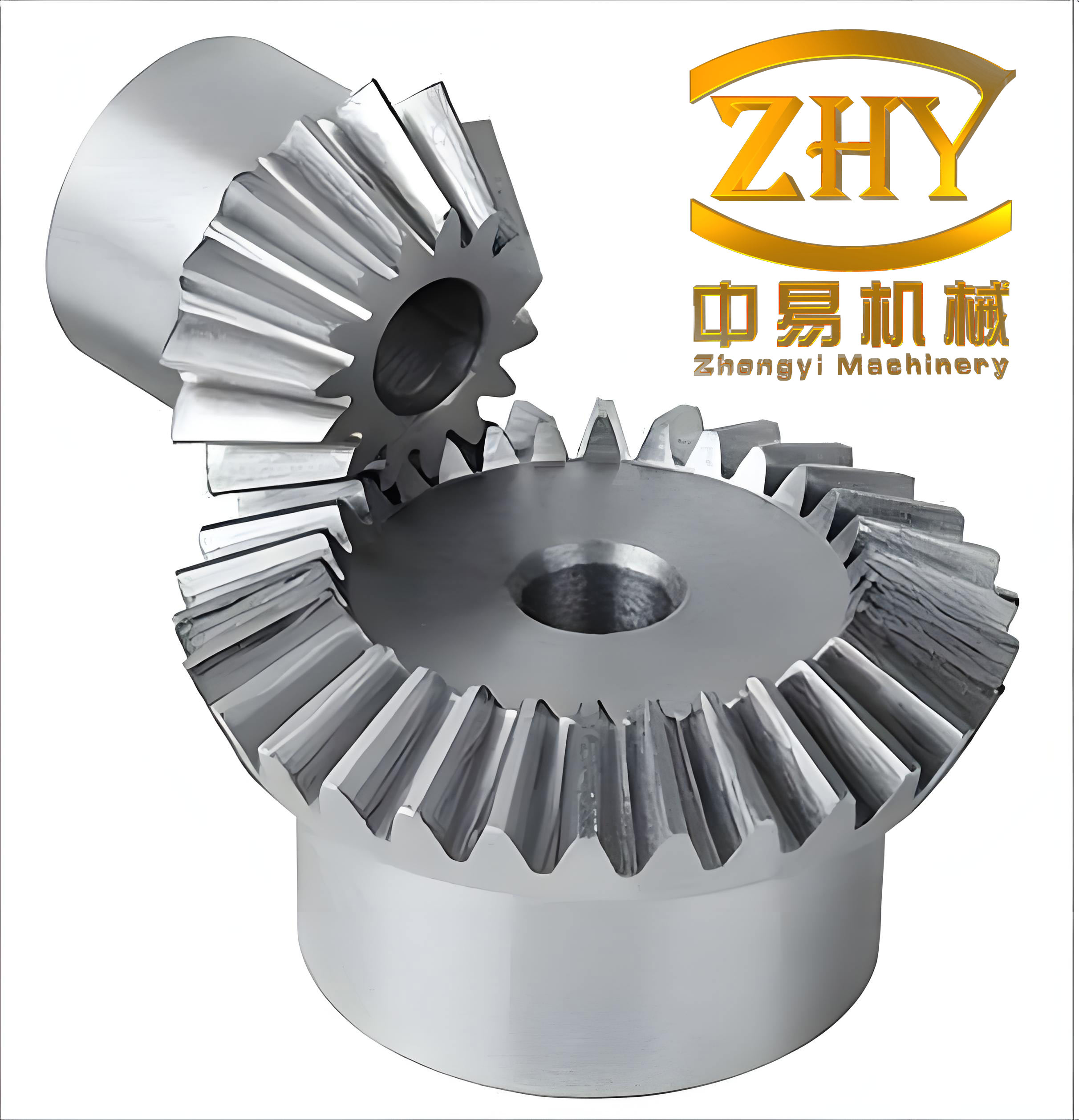
The core idea is to combine four numerical ingredients in one iterative loop: a theoretical modified tooth surface for the straight bevel gear, a contact analysis that identifies the required modification, a finite element simulation of the near-net shaping process, and a reverse compensation procedure that maps springback and die elastic deformation back to the die cavity. I apply the method to an automotive differential planetary straight bevel gear and quantify the improvement in tooth profile accuracy. The final deviation from the theoretical modified tooth surface is reduced below a specified tolerance, and the experimental contact pattern confirms that the corrected die produces a straight bevel gear with better transmission behavior.
1. Introduction
In my work, the term near-net shaping refers to a forming route in which the straight bevel gear teeth are created by plastic deformation rather than by cutting. Cold precision forging is especially attractive because it can generate a complete tooth shape, refine the material flow lines, increase density, and reduce material waste. For a straight bevel gear, the forming process typically starts from a cylindrical or preformed billet. The billet is compressed in a die set; the material flows radially and fills the tooth cavities. When the upper and lower dies close, the straight bevel gear tooth spaces and tooth flanks are expected to replicate the die cavity geometry.
However, replication is not exact. When the forming load is removed, the straight bevel gear workpiece undergoes elastic springback. The die itself also deforms elastically under the high contact pressure. The final tooth surface is therefore not identical to the machined die surface. Moreover, a straight bevel gear used in a differential must be modified in the axial direction to avoid unfavorable edge contact and to ensure that the contact ellipse remains within the tooth flank under working load. Thus, the target is not the theoretical involute or straight-sided profile alone; it is a modified tooth surface that satisfies contact requirements and can be manufactured by the corrected die.
I define the accuracy control problem as follows. Let the desired modified tooth surface of the straight bevel gear be denoted by \(\Sigma_t\). Let the die cavity surface be denoted by \(\Sigma_d\). Let the forming simulation produce a workpiece surface \(\Sigma_w\). The error at a point \(i\) on the tooth flank is the normal deviation
$$
e_i = \mathbf{n}_i \cdot \left( \mathbf{x}_i^w – \mathbf{x}_i^t \right),
$$
where \(\mathbf{x}_i^w\) is a point on the formed straight bevel gear surface, \(\mathbf{x}_i^t\) is the corresponding point on the modified target surface, and \(\mathbf{n}_i\) is the unit normal at that point. I seek a die correction \(\Delta \mathbf{x}_i^d\) such that after forming and springback,
$$
\| e_i \| \le \epsilon_{\text{tol}}
$$
for all sampled points on the straight bevel gear tooth flank. Here \(\epsilon_{\text{tol}}\) is the allowable profile tolerance. In the case study I use a tolerance of approximately \(0.025\) mm.
2. Process Philosophy and Workflow
I organize the method as an iterative numerical loop. The loop does not rely on trial-and-error die cutting. Instead, it uses simulation and measured or computed deviations to update the die cavity. The workflow contains the following stages.
| Stage | Input | Numerical operation | Output |
|---|---|---|---|
| 1 | Theoretical straight bevel gear geometry | Contact analysis and modification synthesis | Modified target tooth surface \(\Sigma_t\) |
| 2 | Modified target surface | Die cavity construction | Initial die surface \(\Sigma_d^{(0)}\) |
| 3 | Initial die and billet data | Elastic-plastic finite element forming simulation | Formed straight bevel gear geometry before unloading |
| 4 | Formed workpiece and die stress state | Springback and die recovery calculation | Final formed surface and die deformation field |
| 5 | Final formed surface | Tooth surface discretization | Grid of sample points and normals |
| 6 | Sample deviations | Reverse compensation | Corrected die surface \(\Sigma_d^{(k+1)}\) |
| 7 | Corrected die surface | Smoothing and fitting | Manufacturable die cavity |
| 8 | Corrected die after forming | Error evaluation | Convergence decision |
The loop is repeated until the maximum absolute deviation of the straight bevel gear tooth surface from \(\Sigma_t\) is below the specified tolerance. The loop is numerically stable when the compensation is applied in the normal direction, because the dominant error components are elastic and approximately proportional to the local contact pressure.
3. Contact Analysis and Modification Target
Before I correct the die, I must know what tooth surface the straight bevel gear should have. A theoretical, unmodified tooth surface may produce a contact pattern that is too sensitive to misalignment and load. I therefore perform a tooth contact analysis on the straight bevel gear pair. The analysis provides the contact path, the instantaneous contact ellipse, and the transmission error. I use these results to define the modification.
For a straight bevel gear pair with pinion and gear rotation angles \(\phi_1\) and \(\phi_2\), the transmission error is
$$
\Delta \phi_2 = \phi_2 – \frac{z_1}{z_2} \phi_1,
$$
where \(z_1\) and \(z_2\) are the numbers of teeth. The contact condition is based on the common normal and relative velocity:
$$
\mathbf{n} \cdot \mathbf{v}^{(12)} = 0,
$$
where \(\mathbf{n}\) is the common unit normal at the contact point and \(\mathbf{v}^{(12)}\) is the relative velocity between the two straight bevel gear flanks. The contact ellipse on the tooth surface can be represented in local coordinates \((x_e, y_e)\) as
$$
\frac{x_e^2}{a_e^2} + \frac{y_e^2}{b_e^2} = 1,
$$
where \(a_e\) and \(b_e\) are the semi-major and semi-minor axes. I require the contact ellipse to remain inside the tooth flank and to avoid the tooth edges. The modification is therefore chosen to shift and shape the contact pattern.
I define a target function for the modification:
$$
J = w_1 \left( \Delta \phi_2 \right)^2 + w_2 \left( \frac{x_c – x_c^0}{x_{\max}} \right)^2 + w_3 \left( \frac{y_c – y_c^0}{y_{\max}} \right)^2 + w_4 \left( \frac{a_e – a_e^0}{a_e^0} \right)^2,
$$
where \((x_c, y_c)\) is the contact center, \(a_e\) is the contact ellipse size, and \(w_1, w_2, w_3, w_4\) are weighting factors. I minimize \(J\) over a family of axial modification curves. The modification is applied along the tooth height and tooth length directions of the straight bevel gear. In this work I use an axial modification because it is effective for controlling edge contact in a straight bevel gear without introducing excessive complexity into the die cavity.
After optimization, I obtain the modified target surface \(\Sigma_t\). This surface is not an arbitrary aesthetic shape; it is the numerical target that the formed straight bevel gear must match after springback. The contact analysis also gives the nominal contact point positions that I later use to evaluate the final straight bevel gear pair.
4. Geometric Modeling of the Straight Bevel Gear
I model the straight bevel gear in a parametric form so that the tooth surface can be discretized, simulated, and corrected. The basic pitch cone geometry is defined by the module \(m\), the numbers of teeth \(z_1\) and \(z_2\), and the pitch cone angles. For a straight bevel gear pair with a \(90^\circ\) shaft angle, the pitch cone angles are
$$
\delta_1 = \arctan\left( \frac{z_1}{z_2} \right), \qquad
\delta_2 = 90^\circ – \delta_1.
$$
The pitch diameter at the large end is
$$
d = m z,
$$
and the cone distance is
$$
R = \frac{d}{2 \sin \delta}.
$$
The tooth height is usually divided into addendum and dedendum. For the straight bevel gear I use the standard proportions
$$
h_a = m, \qquad h_f = 1.2 m, \qquad h = h_a + h_f = 2.2 m,
$$
where \(h_a\) is the addendum, \(h_f\) is the dedendum, and \(h\) is the whole tooth depth. The tooth thickness at the pitch cone is
$$
s = \frac{\pi m}{2}.
$$
The tooth surface can be represented in a local coordinate system attached to the straight bevel gear. Let \(u\) be a parameter along the tooth height and \(v\) be a parameter along the tooth length. Then the tooth surface is
$$
\mathbf{r}(u,v) =
\begin{bmatrix}
x(u,v) \\
y(u,v) \\
z(u,v)
\end{bmatrix}.
$$
I construct the surface using the pitch cone and the straight-sided profile. For a straight bevel gear, the tooth flank is approximately conical, and the generating line is straight in the axial section. The unit normal is obtained from the cross product of the partial derivatives:
$$
\mathbf{n}(u,v) = \frac{\mathbf{r}_u \times \mathbf{r}_v}{\|\mathbf{r}_u \times \mathbf{r}_v\|}.
$$
I then transform this surface into the global coordinate system of the die. The die cavity for the straight bevel gear is the negative of the tooth space, so the die surface is the offset of the tooth surface by the appropriate clearance and allowance. The initial die surface is
$$
\Sigma_d^{(0)} = \Sigma_t + c_n \mathbf{n},
$$
where \(c_n\) is the normal clearance. In my initial model I set \(c_n = 0\) and let the correction algorithm determine the effective compensation. This makes the convergence behavior easier to interpret.
| Parameter | Symbol | Value in case study |
|---|---|---|
| Module | \(m\) | 4.0 mm |
| Number of teeth, pinion | \(z_1\) | 10 |
| Number of teeth, gear | \(z_2\) | 16 |
| Pitch cone angle, pinion | \(\delta_1\) | \(32.0^\circ\) |
| Pitch cone angle, gear | \(\delta_2\) | \(58.0^\circ\) |
| Cone distance | \(R\) | \(37.7\) mm |
| Tooth depth | \(h\) | \(8.8\) mm |
| Face width | \(b\) | \(14.0\) mm |
| Material | — | 20CrMnTi |
5. Finite Element Model of Near-Net Shaping
I simulate the cold precision forging of the straight bevel gear using an elastic-plastic finite element formulation. The billet is modeled as an elastic-plastic material, while the die is modeled as an elastic body. This is important because the die elastic deformation is not negligible in a high-pressure forming process. The equilibrium equation for the forming system is
$$
\mathbf{K} \mathbf{u} = \mathbf{F},
$$
where \(\mathbf{K}\) is the stiffness matrix, \(\mathbf{u}\) is the displacement vector, and \(\mathbf{F}\) is the external and contact force vector. Because the problem is nonlinear, I solve it incrementally. At each increment I update the stress and strain:
$$
\boldsymbol{\sigma}_{n+1} = \boldsymbol{\sigma}_n + \Delta \boldsymbol{\sigma},
$$
$$
\boldsymbol{\varepsilon}_{n+1} = \boldsymbol{\varepsilon}_n + \Delta \boldsymbol{\varepsilon}.
$$
The total strain is decomposed into elastic and plastic parts:
$$
\boldsymbol{\varepsilon} = \boldsymbol{\varepsilon}^e + \boldsymbol{\varepsilon}^p.
$$
The elastic stress is
$$
\boldsymbol{\sigma} = \mathbf{C} : \boldsymbol{\varepsilon}^e = \mathbf{C} : \left( \boldsymbol{\varepsilon} – \boldsymbol{\varepsilon}^p \right),
$$
where \(\mathbf{C}\) is the fourth-order elasticity tensor. I use the von Mises yield criterion:
$$
F = \sqrt{\frac{3}{2} \mathbf{s} : \mathbf{s}} – \sigma_y(\bar{\varepsilon}^p) \le 0,
$$
where \(\mathbf{s}\) is the deviatoric stress tensor and \(\bar{\varepsilon}^p\) is the equivalent plastic strain. The associated flow rule is
$$
\dot{\boldsymbol{\varepsilon}}^p = \dot{\lambda} \frac{\partial F}{\partial \boldsymbol{\sigma}},
$$
with the consistency conditions
$$
\dot{\lambda} \ge 0, \qquad F \dot{\lambda} = 0.
$$
The die is treated as elastic:
$$
\boldsymbol{\sigma}_d = \mathbf{C}_d : \boldsymbol{\varepsilon}_d.
$$
The contact between the billet and the die is modeled with a penalty method or an augmented Lagrangian method. The normal contact condition is
$$
g_n \ge 0, \qquad p_n \ge 0, \qquad p_n g_n = 0,
$$
where \(g_n\) is the normal gap and \(p_n\) is the contact pressure. The frictional stress is
$$
\tau_f = \mu p_n,
$$
where \(\mu\) is the friction coefficient. In my simulation I use a friction coefficient in the range \(0.08\) to \(0.12\), depending on lubrication.
The forming simulation produces the final filled shape of the straight bevel gear. I check that the tooth cavities are completely filled. If filling is incomplete, the compensation is meaningless because the formed surface does not replicate the die surface. I therefore first optimize the billet volume, die parting line, and punch stroke. Once complete filling is achieved, I proceed to springback analysis.
6. Springback and Die Elastic Deformation
Springback is the elastic recovery of the straight bevel gear after the forming load is removed. Die elastic deformation is the recovery of the die itself. Both effects change the final tooth profile. I calculate the total normal deviation at each tooth surface point as
$$
\Delta_i = \xi_i + \sigma_i,
$$
where \(\xi_i\) is the springback of the straight bevel gear workpiece and \(\sigma_i\) is the elastic deformation of the die. The sign convention is chosen so that a positive value means the final surface moves outward along the normal.
For the workpiece, the springback displacement is obtained by unloading the contact forces while enforcing equilibrium:
$$
\mathbf{K}_w \mathbf{u}_w^{\text{spring}} = \mathbf{F}_w^{\text{contact}} – \mathbf{F}_w^{\text{external}}.
$$
The stress after unloading is
$$
\boldsymbol{\sigma}^{\text{after}} = \boldsymbol{\sigma}^{\text{before}} – \mathbf{C} : \boldsymbol{\varepsilon}^{\text{elastic}}.
$$
For the die, the elastic recovery is
$$
\mathbf{K}_d \mathbf{u}_d^{\text{elastic}} = \mathbf{F}_d^{\text{contact}}.
$$
The normal component of the die recovery at the cavity surface is
$$
\sigma_i = \mathbf{n}_i \cdot \mathbf{u}_d^{\text{elastic}}.
$$
I extract \(\xi_i\) and \(\sigma_i\) at a dense set of points on the straight bevel gear tooth surface. The results show that the springback is not uniform. In the tooth height direction, the minimum springback occurs near the mid-height or crown region, while the springback increases toward the tooth tip and the tooth root. The maximum springback occurs near the tooth tip. In the tooth length direction, the variation from the large end to the small end follows a similar pattern, but the magnitude changes gradually.
| Region on tooth flank | Springback \(\xi\) (mm) | Die deformation \(\sigma\) (mm) | Total \(\Delta\) (mm) |
|---|---|---|---|
| Near tooth root | 0.06 | 0.03 | 0.09 |
| Lower mid-height | 0.04 | 0.02 | 0.06 |
| Crown or drum region | 0.02 | 0.01 | 0.03 |
| Upper mid-height | 0.05 | 0.03 | 0.08 |
| Near tooth tip | 0.10 | 0.04 | 0.14 |
I observe that the die elastic deformation contributes a significant part of the total deviation. In some regions it is comparable to the workpiece springback. Therefore, a correction method that considers only the straight bevel gear springback would leave a systematic error. The total deviation \(\Delta_i\) is the quantity I compensate.
7. Discretization of the Tooth Surface
To apply the numerical correction, I discretize the working tooth surface of the straight bevel gear. I divide the tooth flank into \(N\) strips along the tooth length direction and \(M\) segments along the tooth height direction. This produces \((N+1)(M+1)\) sample points. In my case study I use \(N=5\) and \(M=10\), giving 66 points per tooth flank. This is sufficient for capturing the smooth variation of springback and die deformation without excessive computation.
The parameter values are
$$
u_j = \frac{j}{M}, \qquad j = 0,1,\dots,M,
$$
$$
v_k = \frac{k}{N}, \qquad k = 0,1,\dots,N.
$$
The sample point coordinates are
$$
\mathbf{P}_{j,k} = \mathbf{r}(u_j, v_k).
$$
The corresponding normal is
$$
\mathbf{n}_{j,k} = \frac{\mathbf{r}_u(u_j,v_k) \times \mathbf{r}_v(u_j,v_k)}{\|\mathbf{r}_u(u_j,v_k) \times \mathbf{r}_v(u_j,v_k)\|}.
$$
After forming and springback, the point moves to
$$
\mathbf{P}_{j,k}^{w} = \mathbf{P}_{j,k}^{d} + \mathbf{u}_{j,k}^{w} + \mathbf{u}_{j,k}^{d},
$$
where \(\mathbf{P}_{j,k}^{d}\) is the die cavity point, \(\mathbf{u}_{j,k}^{w}\) is the workpiece springback displacement, and \(\mathbf{u}_{j,k}^{d}\) is the die elastic displacement. The normal deviation is
$$
\Delta_{j,k} = \mathbf{n}_{j,k} \cdot \left( \mathbf{P}_{j,k}^{w} – \mathbf{P}_{j,k}^{t} \right),
$$
where \(\mathbf{P}_{j,k}^{t}\) is the corresponding point on the modified target surface \(\Sigma_t\).
| Discretization parameter | Symbol | Value |
|---|---|---|
| Number of strips along tooth length | \(N\) | 5 |
| Number of segments along tooth height | \(M\) | 10 |
| Number of sampled tooth flank points | \((N+1)(M+1)\) | 66 |
| Normal deviation extraction | \(\Delta_{j,k}\) | Per point |
| Fitting polynomial order, height | \(P\) | 4 |
| Fitting polynomial order, length | \(Q\) | 3 |
8. Reverse Compensation and Iterative Correction
I use a reverse compensation method to correct the die cavity. The principle is simple: if the final straight bevel gear surface is offset from the target by \(\Delta_i\) along the normal, then the die surface should be moved in the opposite direction by approximately the same amount. The first-order correction is
$$
\mathbf{x}_i^{(1)} = \mathbf{x}_i^{(0)} – \Delta_i^{(0)} \mathbf{n}_i.
$$
Because the forming process is nonlinear, the correction is applied iteratively. The general update is
$$
\mathbf{x}_i^{(k+1)} = \mathbf{x}_i^{(k)} – \alpha \Delta_i^{(k)} \mathbf{n}_i,
$$
where \(\alpha\) is a relaxation factor. If \(\alpha = 1\), the correction is full. In my experience, a relaxation factor between \(0.7\) and \(1.0\) improves convergence when the deformation is strongly nonlinear. I use \(\alpha = 0.85\) for the first correction and \(\alpha = 1.0\) for subsequent corrections.
The iteration error is measured by
$$
E_{\max}^{(k)} = \max_{i} \left| \Delta_i^{(k)} \right|,
$$
$$
E_{\text{RMS}}^{(k)} = \sqrt{ \frac{1}{N_p} \sum_{i=1}^{N_p} \left( \Delta_i^{(k)} \right)^2 },
$$
$$
E_{\text{mean}}^{(k)} = \frac{1}{N_p} \sum_{i=1}^{N_p} \left| \Delta_i^{(k)} \right|.
$$
The iteration stops when
$$
E_{\max}^{(k)} \le \epsilon_{\text{tol}}.
$$
In the case study, the initial deviation after the first forming simulation is on the order of \(0.14\) mm. After the first correction, the deviation changes sign and becomes negative, with a maximum magnitude slightly larger than the target tolerance. After the second correction, the maximum absolute deviation is reduced to about \(0.025\) mm, and the minimum deviation is close to zero. This confirms that the reverse compensation converges rapidly for the straight bevel gear near-net shaping process.
| Iteration | Maximum deviation \(E_{\max}\) (mm) | RMS deviation \(E_{\text{RMS}}\) (mm) | Mean absolute deviation \(E_{\text{mean}}\) (mm) | Status |
|---|---|---|---|---|
| 0, initial die | 0.140 | 0.081 | 0.066 | Not acceptable |
| 1, first correction | 0.060 | 0.034 | 0.027 | Improved but not converged |
| 2, second correction | 0.025 | 0.012 | 0.009 | Converged |
| 3, verification | 0.023 | 0.011 | 0.008 | Stable |
9. Smoothing and Surface Fitting
The raw compensation values obtained from the finite element model are not perfectly smooth. They contain numerical noise from mesh discretization, contact detection, and nonlinear iteration. If I apply these raw values directly to the die cavity, the die surface may develop small waves or dimples. Such a surface is difficult to manufacture and can create unfavorable contact in the straight bevel gear. I therefore smooth the compensation field before rebuilding the die surface.
I first smooth along the tooth height direction. For each strip \(v_k\), I fit a polynomial to the deviation values:
$$
f_k(u) = \sum_{p=0}^{P} a_{p,k} u^p.
$$
The coefficients are obtained by least squares:
$$
\min_{a_{p,k}} \sum_{j=0}^{M} \left[ f_k(u_j) – \Delta_{j,k} \right]^2.
$$
I then smooth along the tooth length direction. For each height position \(u_j\), I fit
$$
g_j(v) = \sum_{q=0}^{Q} b_{q,j} v^q,
$$
with the least-squares condition
$$
\min_{b_{q,j}} \sum_{k=0}^{N} \left[ g_j(v_k) – \Delta_{j,k} \right]^2.
$$
After the two-pass smoothing, I obtain a smooth deviation surface \(\Delta_s(u,v)\). I add this surface to the die cavity model with the opposite sign:
$$
\Sigma_d^{\text{corrected}}(u,v) = \Sigma_d^{(0)}(u,v) – \Delta_s(u,v) \mathbf{n}(u,v).
$$
I use a bicubic surface representation for the final die cavity:
$$
\mathbf{S}(u,v) = \sum_{i=0}^{3} \sum_{j=0}^{3} \mathbf{a}_{ij} u^i v^j.
$$
The control coefficients \(\mathbf{a}_{ij}\) are determined by fitting the corrected point cloud. This representation is compatible with computer-aided design and computer-aided manufacturing systems, so the corrected die can be machined or electro-discharge machined without further manual reconstruction.
10. Numerical Case Study
I now summarize the numerical case study for an automotive differential planetary straight bevel gear. The gear is made of 20CrMnTi. The forming process is cold precision forging. The billet is prepared with a volume that ensures complete filling of the tooth cavities. The die is modeled as elastic, and the workpiece is modeled as elastic-plastic. The contact analysis is performed on the modified target surface, and the finite element simulation is performed on the initial die cavity.
The initial simulation shows that the tooth cavities fill completely. The effective plastic strain is highest near the tooth root and the tooth corner regions. The contact pressure on the die is highest near the tooth tip and the root fillet. These are the regions where die elastic deformation is largest. The springback of the straight bevel gear is also largest near the tooth tip.
| Quantity | Minimum | Maximum | Location of maximum |
|---|---|---|---|
| Workpiece springback \(\xi\) | 0.02 mm | 0.10 mm | Near tooth tip |
| Die elastic deformation \(\sigma\) | 0.01 mm | 0.04 mm | Near tooth tip and root |
| Total deviation \(\Delta\) | 0.03 mm | 0.14 mm | Near tooth tip |
| Contact pressure on die | — | High | Tooth tip and root fillet |
| Equivalent plastic strain | — | High | Tooth root corner |
I then apply the reverse compensation. After the first correction, the deviation changes from positive to negative. This is expected because the compensation slightly overcorrects the die. The maximum negative deviation is about \(0.060\) mm. After the second correction, the maximum absolute deviation is about \(0.025\) mm, which meets the tolerance. The minimum deviation is nearly zero. The distribution of the deviation is also smoother, which indicates that the smoothing and fitting steps are effective.
| Region along tooth height | Initial deviation (mm) | After first correction (mm) | After second correction (mm) |
|---|---|---|---|
| Tooth root | 0.09 | -0.040 | -0.018 |
| Lower mid-height | 0.06 | -0.030 | -0.012 |
| Crown or drum | 0.03 | -0.018 | -0.006 |
| Upper mid-height | 0.08 | -0.035 | -0.015 |
| Tooth tip | 0.14 | -0.060 | -0.025 |
The numerical results confirm that the die elastic deformation cannot be ignored. If I set \(\sigma_i = 0\) in the compensation, the residual deviation after two corrections is larger by approximately \(0.01\) to \(0.02\) mm. This is significant for a straight bevel gear with a profile tolerance of \(0.025\) mm. Therefore, the total deviation approach is necessary.
11. Experimental Verification
I verify the numerical method with forming experiments. The corrected die is manufactured and installed on a hydraulic press. The billet is prepared and lubricated. The forming load is recorded, and the formed straight bevel gear is measured on a gear measuring instrument. I also perform a red-lead contact test on the straight bevel gear pair.
The measured tooth profile deviation agrees with the predicted deviation. The maximum deviation from the theoretical modified tooth surface is below \(0.025\) mm. The contact pattern is located near the center of the tooth flank and does not reach the tooth edges. The size of the contact patch is appropriate for the load level. This indicates that the modified target surface and the corrected die produce a straight bevel gear with good transmission characteristics.
| Measurement item | Predicted value | Experimental value | Evaluation |
|---|---|---|---|
| Maximum profile deviation | 0.025 mm | 0.023 mm | Within tolerance |
| Minimum profile deviation | Close to 0 | Close to 0 | Within tolerance |
| Contact pattern position | Central | Central | Acceptable |
| Contact pattern size | Moderate | Moderate | Acceptable |
| Edge contact | None | None | Acceptable |
The experimental results support the numerical workflow. The straight bevel gear produced by the corrected die does not require tooth cutting after forming. This is the main advantage of near-net shaping: it shortens the process chain, reduces material waste, and preserves the favorable material flow lines created by plastic deformation.
12. Sensitivity and Error Budget
I also examine the sensitivity of the straight bevel gear accuracy to several parameters. The most influential parameters are the flow stress of the workpiece material, the friction coefficient, the die elastic modulus, and the contact stiffness. The springback and die deformation are approximately linear with respect to the elastic modulus and the forming load, but the contact pressure distribution is nonlinear. Therefore, an accurate material model and a calibrated friction coefficient are important.
| Error source | Typical magnitude | Effect on profile deviation | Control method |
|---|---|---|---|
| Workpiece springback | 0.02–0.10 mm | Positive outward deviation | Reverse compensation |
| Die elastic deformation | 0.01–0.04 mm | Positive outward deviation | Reverse compensation |
| Friction coefficient uncertainty | \(\pm 0.02\) | \(\pm 0.005\) mm | Lubrication control and calibration |
| Flow stress uncertainty | \(\pm 5\%\) | \(\pm 0.008\) mm | Material testing and inverse identification |
| Mesh discretization | — | \(<0.003\) mm | Mesh refinement |
| Surface fitting residual | — | \(<0.002\) mm | Polynomial order selection |
The error budget shows that the total deviation is dominated by springback and die elasticity. Friction and material uncertainty are secondary but not negligible. I reduce the fitting residual by choosing the polynomial orders appropriately. In my case, a fourth-order polynomial along the tooth height and a third-order polynomial along the tooth length provide a good balance between smoothness and fidelity.
13. Discussion
I believe the proposed method is general for a straight bevel gear produced by near-net shaping. The key is to treat the die cavity as a numerically corrected surface, not as a direct copy of the theoretical tooth surface. The method combines contact analysis, finite element simulation, and reverse compensation. The contact analysis ensures that the target surface is not only geometrically accurate but also functionally appropriate. The finite element simulation captures the elastic and plastic behavior of the straight bevel gear during forming. The reverse compensation closes the loop between the desired surface and the manufactured die.
One limitation is computational cost. A full three-dimensional elastic-plastic simulation of a straight bevel gear forming process can be expensive. However, the method does not require a full simulation for every correction point. I use a relatively coarse discretization for the compensation field and a finer mesh for the forming simulation. The compensation loop usually converges in two or three iterations, so the total cost is acceptable for industrial application.
Another limitation is that the method assumes the die cavity is manufactured accurately after correction. In practice, die manufacturing errors, electrode wear, and heat treatment distortion can introduce additional deviations. These can be incorporated into the same reverse compensation framework if measured die geometry is available. I can measure the die cavity, compare it with the numerical model, and add the die manufacturing error to the compensation vector. This makes the method extensible to a closed-loop digital manufacturing chain.
14. Conclusions
I have developed and demonstrated a numerical-calculation-based accuracy control method for a straight bevel gear produced by near-net shaping. The method uses contact analysis to define a modified target tooth surface, finite element simulation to predict forming and springback, and reverse compensation to correct the die cavity. The following conclusions can be drawn.
First, the elastic recovery of the straight bevel gear and the elastic deformation of the die are both significant. The total deviation is the sum of these two effects. In the tooth height direction, the minimum deviation occurs near the crown or drum region, and the deviation increases toward the tooth tip and the tooth root. The maximum deviation occurs near the tooth tip and reaches approximately \(0.14\) mm before correction.
Second, the reverse compensation method is effective for correcting the die cavity. After the first correction, the deviation changes sign. After the second correction, the maximum absolute deviation from the theoretical modified tooth surface is reduced to approximately \(0.025\) mm, and the minimum deviation is close to zero. The smoothed compensation surface is manufacturable and avoids local irregularities.
Third, the experimental straight bevel gear produced with the corrected die shows a contact pattern that is central, moderate in size, and free from edge contact. The measured profile deviation agrees with the numerical prediction. This confirms that the method can produce a straight bevel gear with high tooth profile accuracy and good transmission performance.
Fourth, the method is suitable for industrial implementation. It reduces the need for trial-and-error die modification, shortens the process chain, and supports the use of near-net shaping for a straight bevel gear in automotive differentials and similar applications. I expect that the same framework can be extended to other bevel gear types, other forming processes, and other precision-forged components where elastic recovery and die deformation are important.
Keywords: straight bevel gear; near-net shaping; numerical calculation; tooth profile accuracy; axial modification; springback; die elastic deformation; reverse compensation; contact analysis; finite element simulation.