
In the realm of gear manufacturing, precision in gear cutting is paramount, especially for non-standard gear types like circular arc gears. As a researcher deeply involved in gear design and production, I have observed that the control of cutting depth during gear cutting processes is a critical factor influencing the performance and longevity of circular arc gears. Unlike involute gears, circular arc gears exhibit superior load-bearing capacity and compact size, but they are highly sensitive to errors in the center distance of transmission. This sensitivity stems from their point-contact meshing mechanism, where slight deviations can drastically reduce contact strength. Therefore, optimizing the control of cutting depth in gear cutting is not just a manufacturing detail but a fundamental requirement for achieving high-performance circular arc gear transmissions. This article delves into the mathematical foundations, practical relationships, and optimization strategies for controlling cutting depth in circular arc gear cutting, leveraging equations, numerical methods, and tabular summaries to provide a comprehensive guide.
Circular arc gears, often referred to as Novikov gears, operate on a point-contact system where meshing occurs along a spatial helix on the tooth surface. This design leads to a larger composite radius of curvature at the contact point compared to involute gears, resulting in higher contact strength as per Hertzian stress theory. However, this advantage comes with a caveat: circular arc gears lack the “separability” characteristic of involute gears, meaning that any deviation from the designed center distance—often caused by errors in gear cutting depth—can lead to misalignment and rapid degradation in load capacity. Thus, in gear cutting operations, whether using hobbing or grinding processes, precise control of the cutting depth is essential to ensure that the actual gear profile matches the theoretical design. The challenge lies in relating measurable parameters, such as chordal tooth thickness, to the cutting depth error, and then using this relationship to adjust the gear cutting process for optimal results.
To address this, I start with the general tooth surface equation for circular arc gears. Derived from the envelope principle, the tooth surface can be represented as a helical surface with specific geometric parameters. Let’s consider a right-handed coordinate system where the z-axis coincides with the gear’s rotational axis, and the tooth symmetry line aligns with the x-axis. The tooth surface equation for a circular arc gear, based on the standard rack profile, is given by:
$$ \vec{r}(u, \theta) = \begin{bmatrix} x(u, \theta) \\ y(u, \theta) \\ z(u, \theta) \end{bmatrix} = \begin{bmatrix} \rho \cos(\alpha + u) + a \\ \rho \sin(\alpha + u) + b \\ p(\theta – u) \end{bmatrix} $$
Here, \( \rho \) is the radius of the circular arc segment in the standard rack, \( \alpha \) is the pressure angle, \( u \) is a parameter along the arc, \( \theta \) is the rotational parameter, \( a \) and \( b \) are the coordinates of the arc’s center in the rack profile, and \( p \) is the spiral parameter defined as \( p = r_b \tan(\beta) \), where \( r_b \) is the base radius and \( \beta \) is the helix angle. This equation describes a helical surface that forms the basis for further analysis in gear cutting. The derivation assumes an ideal gear cutting process with no errors, but in reality, deviations occur, particularly in cutting depth, which we must account for.
In gear cutting, the cutting depth directly influences the position of the tooth profile relative to the gear blank. When there is an error in cutting depth, denoted as \( \Delta h \), it corresponds to a shift in the rack profile’s position. This shift can be incorporated into the tooth surface equation by modifying the center coordinates. Specifically, if the cutting depth error is positive (i.e., cutting too deep), the rack profile moves inward, altering the tooth geometry. To quantify this, we define a “cutting depth variation coefficient” \( k \), which relates the error to the rack’s y-coordinate. In the modified equation, the y-coordinate of the arc center becomes \( b + k \), where \( k \) is proportional to \( \Delta h \). This adjustment allows us to model the actual tooth surface after gear cutting with depth errors.
The core of controlling gear cutting depth lies in the relationship between chordal tooth thickness and cutting depth error. Chordal tooth thickness, measured at a specific height from the tooth tip, is a common metric in gear inspection. For circular arc gears, the theoretical chordal thickness is calculated at the point where the pressure angle equals the nominal pressure angle, but due to errors in gear cutting, the actual measurement point may differ. To establish the relationship, consider two helical lines on the tooth surface representing the contact paths. The chordal thickness \( \bar{s} \) is the shortest distance between these lines, and it can be derived by solving an optimization problem for the parameter \( u \). The governing equation for \( u \) is:
$$ \frac{\partial}{\partial u} \left[ \left( x_1(u_1, \theta_1) – x_2(u_2, \theta_2) \right)^2 + \left( y_1(u_1, \theta_1) – y_2(u_2, \theta_2) \right)^2 + \left( z_1(u_1, \theta_1) – z_2(u_2, \theta_2) \right)^2 \right] = 0 $$
Where subscripts 1 and 2 refer to the two helical lines. Solving this yields the specific \( u \) value that minimizes the distance, and substituting back gives the chordal thickness. The corresponding measurement height \( \bar{h} \) is calculated based on the tooth tip geometry. However, when gear cutting errors exist, the measured chordal thickness \( \bar{s}’ \) will deviate from the theoretical value \( \bar{s} \). This deviation is linked to the cutting depth error through the coefficient \( k \). The relationship can be expressed as an implicit function:
$$ F(\bar{s}’, k, \alpha) = 0 $$
Where \( \alpha \) is the pressure angle at the measurement point. Solving this equation allows us to determine \( k \) and, consequently, the cutting depth error \( \Delta h \). This forms the basis for optimizing gear cutting processes.
In practice, gear cutting involves multiple parameters, and the relationship between chordal thickness and cutting depth error is nonlinear. To handle this, I employ optimization techniques and numerical methods. The goal is to find the value of \( k \) that minimizes the difference between the measured chordal thickness and the theoretical value derived from the tooth surface equation with error. This can be formulated as an equality-constrained optimization problem:
$$ \min_{k, \alpha} \left( \bar{s}’ – \bar{s}(k, \alpha) \right)^2 $$
Subject to: $$ G(k, \alpha) = 0 $$
Where \( G(k, \alpha) \) represents additional constraints from the gear geometry, such as the tooth tip diameter or helix angle. Using methods like the damped least-squares approach or modified quadratic approximation, we can solve for \( k \) efficiently. For initial guesses in numerical solutions, when the measured chordal thickness \( \bar{s}’ \) equals the theoretical value \( \bar{s} \), we have \( k = 0 \) and \( \alpha = \alpha_0 \) (the nominal pressure angle). If \( \bar{s}’ > \bar{s} \), then \( k > 0 \), indicating a need to reduce cutting depth in gear cutting, and vice versa. This iterative approach ensures precise control over the gear cutting process.
To illustrate, let’s consider a numerical example for a double circular arc gear. Assume the following parameters from a standard rack profile: module \( m_n = 4 \, \text{mm} \), number of teeth \( z = 30 \), helix angle \( \beta = 15^\circ \), convex tooth arc radius coefficient \( \rho_a^* = 1.2 \), addendum coefficient \( h_a^* = 0.8 \), convex tooth arc center offset coefficient \( e_a^* = 0.25 \), shift coefficient \( x = 0.1 \), and nominal pressure angle \( \alpha_0 = 20^\circ \). Using these, we compute the theoretical fixed chordal thickness \( \bar{s} \) and fixed chordal height \( \bar{h} \). Then, for a measured chordal thickness \( \bar{s}’ \), we solve for \( k \) and \( \Delta h \). The results can be plotted as curves showing the relationship between \( \bar{s}’ \), \( k \), and \( \Delta h \), which are crucial for adjusting gear cutting depth.
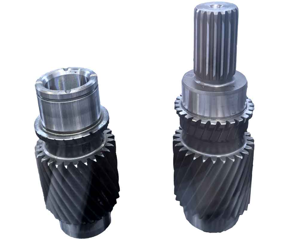
The image above illustrates a typical setup in gear cutting for circular arc gears, highlighting the importance of precision in tool positioning and depth control. Such visual aids reinforce the practical aspects of the optimization methods discussed.
For a more structured summary, I present key formulas and relationships in tables. These tables encapsulate the mathematical foundations essential for gear cutting control.
| Parameter | Symbol | Description | Typical Value or Formula |
|---|---|---|---|
| Arc radius | \( \rho \) | Radius of circular arc in rack profile | \( \rho = \rho^* m_n \) |
| Spiral parameter | \( p \) | Helical motion parameter | \( p = r_b \tan(\beta) \) |
| Center coordinates | \( a, b \) | Coordinates of arc center in rack | Defined by rack geometry |
| Cutting depth variation coefficient | \( k \) | Relates to cutting depth error \( \Delta h \) | \( k = c \cdot \Delta h \), where \( c \) is a constant |
| Pressure angle | \( \alpha \) | Angle at measurement point | May deviate from \( \alpha_0 \) due to errors |
The tooth surface equation is fundamental for simulating gear cutting outcomes. In gear cutting operations like hobbing, the tool geometry must match this equation to generate the desired profile.
| Variable | Symbol | Calculation Method | Notes for Gear Cutting |
|---|---|---|---|
| Theoretical chordal thickness | \( \bar{s} \) | Solved from helical line distance minimization | Based on ideal gear cutting with no errors |
| Measured chordal thickness | \( \bar{s}’ \) | Actual measurement after gear cutting | Includes errors from gear cutting depth |
| Measurement height | \( \bar{h} \) | \( \bar{h} = h_a – \frac{\rho(1 – \cos(u))}{\cos(\alpha)} \) | Dependent on tooth tip diameter |
| Cutting depth error | \( \Delta h \) | Derived from \( k \) via \( \Delta h = k / c \) | Positive \( \Delta h \) means cutting too deep |
| Optimization function | \( F(\bar{s}’, k, \alpha) \) | \( F = \bar{s}’ – \bar{s}(k, \alpha) = 0 \) | Solved numerically to control gear cutting |
These tables emphasize how gear cutting parameters interlink, providing a quick reference for engineers. In gear cutting practice, using these relationships, we can derive correction factors for machine settings.
Now, delving deeper into the optimization process for gear cutting, the numerical solution of the equation \( F(\bar{s}’, k, \alpha) = 0 \) is critical. Since this is a nonlinear equation, direct analytical solutions are impractical. Instead, I use iterative methods. For instance, the Newton-Raphson method can be applied if we compute the Jacobian. Alternatively, for robustness, the Levenberg-Marquardt algorithm (a damped least-squares method) is effective. The objective is to minimize the residual \( R = \bar{s}’ – \bar{s}(k, \alpha) \), considering \( k \) and \( \alpha \) as variables. The iterative update is:
$$ \begin{bmatrix} k_{n+1} \\ \alpha_{n+1} \end{bmatrix} = \begin{bmatrix} k_n \\ \alpha_n \end{bmatrix} – (J^T J + \lambda I)^{-1} J^T R $$
Where \( J \) is the Jacobian matrix of partial derivatives \( \frac{\partial \bar{s}}{\partial k} \) and \( \frac{\partial \bar{s}}{\partial \alpha} \), \( \lambda \) is a damping parameter, and \( I \) is the identity matrix. This approach converges quickly even with poor initial guesses, making it suitable for real-time adjustments in gear cutting.
Moreover, in gear cutting, other errors such as tooth tip diameter deviations can affect chordal thickness measurements. To account for this, we can extend the optimization framework. Let \( \Delta d_a \) be the error in tooth tip diameter. Then, the measurement height \( \bar{h} \) is adjusted, and the chordal thickness calculation incorporates this. The modified relationship becomes:
$$ \bar{s}(k, \alpha, \Delta d_a) = \bar{s}_0(k, \alpha) + \delta(\Delta d_a) $$
Where \( \bar{s}_0 \) is the thickness without tip error, and \( \delta \) is a correction term. By including \( \Delta d_a \) as an input parameter in the optimization, we can isolate the cutting depth error more accurately. This is crucial in high-precision gear cutting for circular arc gears, where cumulative errors must be minimized.
To demonstrate the practical application, consider a gear cutting scenario for a large-diameter circular arc gear. After rough cutting, we measure the chordal thickness at several teeth to account for variations. Suppose the average measured \( \bar{s}’ = 6.35 \, \text{mm} \), and the theoretical \( \bar{s} = 6.40 \, \text{mm} \). Using the optimization method, we solve for \( k \) and find \( \Delta h = -0.02 \, \text{mm} \), indicating that the gear cutting depth is too shallow by 0.02 mm. The machine operator then adjusts the radial feed to increase the cutting depth accordingly. This iterative measurement and adjustment process ensures that the final gear meets design specifications.
The sensitivity of circular arc gears to center distance errors makes gear cutting depth control even more critical. A small error in cutting depth can lead to a significant shift in the meshing point, reducing the contact ellipse size and increasing stress. According to Hertzian contact theory, the contact stress \( \sigma_H \) is inversely proportional to the square root of the composite curvature radius \( \rho_c \):
$$ \sigma_H \propto \frac{1}{\sqrt{\rho_c}} $$
For circular arc gears, \( \rho_c \) is large under ideal conditions, but with cutting depth errors, it decreases rapidly. Therefore, in gear cutting, we aim to minimize \( \Delta h \) to preserve \( \rho_c \). The optimization control directly contributes to this goal by linking measurable thickness to depth errors.
Another aspect of gear cutting for circular arc gears is the use of different manufacturing processes, such as hobbing and grinding. In hobbing, the cutting depth is controlled by the radial infeed of the hob, while in grinding, it involves the wheel position. The mathematical models derived here apply to both, but the implementation may differ. For hobbing, the cutting depth error \( \Delta h \) relates to the machine’s coordinate system, whereas for grinding, it might involve wear compensation. Nonetheless, the core relationship between chordal thickness and cutting depth remains valid, making this approach versatile for gear cutting operations.
To further enrich the discussion, let’s explore the geometric derivation of the chordal thickness formula. The helical lines on the tooth surface are defined by the tooth surface equation with specific parameters. Let \( \vec{r}_1(u, \theta) \) and \( \vec{r}_2(u, \theta) \) represent the two lines for opposite flanks of the same tooth. The distance between them is:
$$ d(u_1, u_2) = \| \vec{r}_1(u_1, \theta_1) – \vec{r}_2(u_2, \theta_2) \| $$
To find the chordal thickness, we minimize \( d \) subject to the constraint that the points lie on the same transverse plane (i.e., \( z_1 = z_2 \)). This leads to \( \theta_1 – u_1 = \theta_2 – u_2 \) due to the helical nature. After simplification, the problem reduces to finding \( u \) that satisfies:
$$ \tan(u) = \frac{p}{r_b} \cdot \frac{\sin(\alpha)}{\cos(\alpha)} $$
This transcendental equation is solved numerically, and the solution \( u^* \) yields the chordal thickness:
$$ \bar{s} = 2 \rho \sin(u^*) \sqrt{1 + \left( \frac{p}{r_b} \right)^2 } $$
This formula shows how gear cutting parameters like \( \rho \) and \( p \) influence the thickness. When cutting depth errors occur, \( \rho \) effectively changes via the coefficient \( k \), altering \( \bar{s} \).
In summary, the control of cutting depth in gear cutting for circular arc gears is a multifaceted problem that combines geometry, optimization, and practical manufacturing. By establishing the tooth surface equation, deriving the chordal thickness relationship, and applying numerical optimization, we can achieve precise control over the gear cutting process. This not only enhances gear performance but also reduces scrap and rework in production.
For a broader perspective, I include a table comparing circular arc gears and involute gears in the context of gear cutting sensitivity.
| Aspect | Circular Arc Gears | Involute Gears | Implications for Gear Cutting |
|---|---|---|---|
| Meshing type | Point contact | Line contact | Circular arc gears require tighter tolerance in gear cutting depth |
| Separability | No | Yes | Gear cutting errors directly affect center distance in circular arc gears |
| Chordal thickness relation | Nonlinear with cutting depth | Linear or simple geometric | Optimization needed for circular arc gear cutting control |
| Typical cutting depth control | Based on chordal thickness measurement and optimization | Based on direct measurement or wire length | Gear cutting for circular arc gears is more computationally intensive |
| Sensitivity to errors | High | Moderate | Demands high precision in gear cutting processes |
This comparison underscores why specialized approaches are necessary for gear cutting of circular arc gears. The optimization methods described here address these unique challenges.
Looking ahead, advancements in gear cutting technology, such as CNC machines and in-process monitoring, can integrate these optimization models for real-time control. For example, during gear cutting, a probe could measure chordal thickness on the fly, and the CNC system could adjust the cutting depth automatically using the algorithms discussed. This would revolutionize the production of high-precision circular arc gears, making gear cutting more efficient and reliable.
In conclusion, the optimization control of cutting depth in circular arc gear manufacturing is essential for leveraging the advantages of these gears while mitigating their sensitivity to errors. Through mathematical modeling, numerical optimization, and practical insights, we can achieve stringent control over the gear cutting process. The relationships and methods outlined here provide a robust framework for engineers and manufacturers to enhance gear quality and performance. As gear cutting evolves, continued refinement of these techniques will drive further improvements in gear technology.
To encapsulate key equations, here is a summary in LaTeX format for quick reference:
$$ \text{Tooth surface: } \vec{r}(u, \theta) = \begin{bmatrix} \rho \cos(\alpha + u) + a \\ \rho \sin(\alpha + u) + b + k \\ p(\theta – u) \end{bmatrix} $$
$$ \text{Chordal thickness: } \bar{s} = 2 \rho \sin(u^*) \sqrt{1 + \left( \frac{p}{r_b} \right)^2 } $$
$$ \text{Optimization: } \min_{k, \alpha} \left( \bar{s}’ – \bar{s}(k, \alpha) \right)^2 $$
$$ \text{Cutting depth error: } \Delta h = \frac{k}{c} $$
These formulas are the backbone of the gear cutting control strategy, enabling precise adjustments and high-quality gear production. By embracing these methods, the gear cutting industry can push the boundaries of what is possible with circular arc gears.