
In the realm of mechanical engineering, gear reducers are pivotal components, and among them, the two-stage helical gear reducer stands out due to its capacity for high load transmission, smooth operation, and compact design. The optimization of such reducers is a complex task, involving numerous design parameters and constraints. In this article, I will delve into a comprehensive optimization design methodology for a two-stage helical gear reducer, focusing on minimizing overall volume while adhering to mechanical integrity criteria. The approach integrates mathematical modeling, parameter normalization, and numerical optimization techniques, with an emphasis on the helical gear’s unique characteristics. Throughout, the term helical gear will be frequently referenced to underscore its central role in this system.
The core objective is to develop an optimal design that reduces material usage and spatial footprint without compromising performance. Traditional design methods often yield feasible but suboptimal solutions; hence, optimization is essential. We establish a mathematical model with design variables, an objective function, and constraints, then solve it using computational methods. This process accounts for real-world intricacies such as discrete variables and empirical coefficients derived from engineering charts.
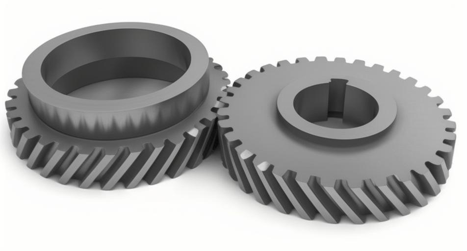
The helical gear, with its angled teeth, offers advantages like increased contact ratio and quieter operation compared to spur gears. However, its design involves additional parameters like helix angle, which complicates optimization. We consider these factors holistically, ensuring that the optimized helical gear reducer meets all mechanical requirements, including strength, durability, and efficiency. The following sections detail the mathematical framework, parameter handling, and a practical example.
Mathematical Model for Optimization
The optimization design of a two-stage helical gear reducer begins with defining the design variables. These variables encapsulate key geometric and operational parameters that influence the system’s performance and size.
Design Variables
We select nine design variables that comprehensively describe the two-stage helical gear reducer. These include parameters for both the high-speed and low-speed stages, ensuring a holistic optimization. The variables are:
- $x_1 = u_1$: Transmission ratio of the high-speed stage helical gear pair.
- $x_2 = z_{11}$: Number of teeth on the pinion of the high-speed stage helical gear.
- $x_3 = m_{n1}$: Normal module of the high-speed stage helical gear.
- $x_4 = \beta_1$: Helix angle of the high-speed stage helical gear (in degrees).
- $x_5 = \phi_{d1}$: Face width coefficient of the high-speed stage helical gear.
- $x_6 = z_{21}$: Number of teeth on the pinion of the low-speed stage helical gear.
- $x_7 = m_{n2}$: Normal module of the low-speed stage helical gear.
- $x_8 = \beta_2$: Helix angle of the low-speed stage helical gear (in degrees).
- $x_9 = \phi_{d2}$: Face width coefficient of the low-speed stage helical gear.
Thus, the design vector is: $$X = [u_1, z_{11}, m_{n1}, \beta_1, \phi_{d1}, z_{21}, m_{n2}, \beta_2, \phi_{d2}]^T$$. These variables are continuous or discrete, requiring special handling during optimization.
Objective Function
The goal is to minimize the total volume, which comprises the gear volumes and the reducer housing volume. This reduces material cost and space. The objective function is a weighted sum of these volumes.
First, the volume of the four helical gears (two pinions and two gears) is approximated using their pitch cylinder volumes: $$f_1(X) = \frac{\pi}{4} (d_{11}^2 b_{11} + d_{12}^2 b_{12} + d_{21}^2 b_{21} + d_{22}^2 b_{22})$$ where $d_{ij}$ and $b_{ij}$ are the pitch diameter and face width of gear $i,j$ (i=1 for high-speed stage, i=2 for low-speed stage; j=1 for pinion, j=2 for gear). For a helical gear, the pitch diameter is calculated as: $$d_{ij} = \frac{m_{ni} z_{ij}}{\cos \beta_i}$$ with $z_{i2} = u_i z_{i1}$ for the gear. The face width is: $$b_{i1} = \phi_{di} d_{i1}$$ and $b_{i2}$ is typically slightly smaller, but for simplicity, we assume $b_{i2} = b_{i1}$ in initial calculations, though adjustments are made in constraints.
Second, the housing volume is modeled as a hollow rectangular box: $$f_2(X) = (l + 2\delta)(b + 2\delta)(h + 2\delta) – l b h$$ where $l$, $b$, and $h$ are internal dimensions, and $\delta$ is the average wall thickness. The internal dimensions are estimated from gear geometry: $$l = d_{12} + d_{21} + d_{11} + d_{22} + 2c_l$$ $$b = b_{12} + b_{21} + c_b$$ $$h = \max(d_{12}, d_{22}) + 2m_{n,\text{max}} + c_h$$ with $c_l$, $c_b$, $c_h$ as constants (e.g., 50 mm, 50 mm, 70 mm). The wall thickness is: $$\delta = \max(0.023(a_1 + a_2) + 3, 8)$$ where $a_i$ is the center distance for stage $i$: $$a_i = \frac{d_{i1} + d_{i2}}{2} = \frac{m_{ni} z_{i1} (1 + u_i)}{2 \cos \beta_i}$$. We adjust $\beta_i$ to make $a_i$ an integer for manufacturability.
The overall objective function is: $$F(X) = w_1 f_1(X) + w_2 f_2(X)$$ where $w_1$ and $w_2$ are weighting factors reflecting the relative importance of gear and housing volumes. Typically, $w_1 = w_2 = 1$ for equal weighting.
Constraint Conditions
The optimization must satisfy multiple constraints to ensure functionality, safety, and manufacturability of the helical gear reducer. These constraints are derived from gear design principles.
1. Transmission Ratio Error: The actual overall ratio must match the desired ratio within a tolerance (e.g., 5%). For a desired total ratio $u$, the constraint is: $$\left| \frac{z_{12} z_{22}}{z_{11} z_{21}} – u \right| \leq 0.05 u$$ where $z_{12} = u_1 z_{11}$ and $z_{22} = u_2 z_{21}$, with $u_2 = \frac{u}{u_1}$.
2. Oil Immersion Depth: To ensure proper lubrication, the low-speed gear should be immersed in oil by about one full tooth height. This leads to: $$d_{22} – d_{12} – 13.5 m_{n2} \leq 0$$ where $13.5 m_{n2}$ approximates twice the tooth height for a helical gear.
3. Contact Ratio: The total contact ratio for each helical gear pair must exceed a minimum value (e.g., 2) for smooth operation. The constraint is: $$\epsilon_{\alpha i} + \epsilon_{\beta i} \geq \epsilon_{0i}, \quad i=1,2$$ where $\epsilon_{\alpha i}$ is the transverse contact ratio, $\epsilon_{\beta i}$ is the axial contact ratio, and $\epsilon_{0i}$ is the required total contact ratio. For helical gears: $$\epsilon_{\alpha i} = \frac{1}{2\pi} \left[ z_{i1} \sqrt{ \left( \frac{r_{ai1}}{r_{i1}} \right)^2 – \cos^2 \alpha_t } + z_{i2} \sqrt{ \left( \frac{r_{ai2}}{r_{i2}} \right)^2 – \cos^2 \alpha_t } – (z_{i1} + z_{i2}) \tan \alpha_t \right]$$ $$\epsilon_{\beta i} = \frac{b_i \sin \beta_i}{\pi m_{ni}}$$ with $\alpha_t$ as the transverse pressure angle: $$\alpha_t = \arctan \left( \frac{\tan \alpha_n}{\cos \beta_i} \right)$$ where $\alpha_n$ is the normal pressure angle (typically 20°).
4. Contact Fatigue Strength: The contact stress for each gear pair must not exceed the allowable stress. For stage $i$, the contact stress is: $$\sigma_{Hi} = Z_H Z_E Z_{\epsilon i} Z_{\beta i} \sqrt{ \frac{2 K_{Hi} T_i (u_i + 1)}{\phi_{di} d_{i1}^3 u_i} }$$ where:
- $Z_H$: Zone factor for helical gears, $$Z_H = \sqrt{ \frac{2 \cos \beta_b}{\cos^2 \alpha_t \tan \alpha_t} }$$ with $\beta_b$ as the base helix angle.
- $Z_E$: Elasticity coefficient, dependent on material properties.
- $Z_{\epsilon i}$: Contact ratio coefficient, $$Z_{\epsilon i} = \sqrt{ \frac{4 – \epsilon_{\alpha i}}{3} }$$ for helical gears.
- $Z_{\beta i}$: Helix angle coefficient, $$Z_{\beta i} = \sqrt{ \cos \beta_i }$$.
- $K_{Hi}$: Load factor for contact stress, $$K_{Hi} = K_A K_{vi} K_{H\alpha} K_{H\beta i}$$ where $K_A$ is application factor, $K_{vi}$ is dynamic factor, $K_{H\alpha}$ is transverse load factor, and $K_{H\beta i}$ is face load factor.
- $T_i$: Torque on pinion, with $T_1$ as input torque and $T_2 = T_1 u_1 \eta$ (considering efficiency $\eta$).
The allowable contact stress for gear $j$ in stage $i$ is: $$[\sigma]_{Hij} = \frac{K_{HNij} \sigma_{Hlimij}}{S_H}$$ where $K_{HNij}$ is life factor, $\sigma_{Hlimij}$ is endurance limit, and $S_H$ is safety factor. Constraints: $$\sigma_{Hi} \leq [\sigma]_{Hij}, \quad i=1,2; j=1,2$$.
5. Bending Fatigue Strength: The bending stress for each gear tooth must be within limits. For gear $j$ in stage $i$: $$\sigma_{Fij} = \frac{2 K_{Fi} T_i Y_{Faij} Y_{Saij} Y_{\epsilon i} Y_{\beta i} \cos \beta_i}{\phi_{di} m_{ni}^3 z_{i1}}$$ where:
- $Y_{Faij}$: Form factor for helical gear, dependent on virtual tooth number $z_{vij} = \frac{z_{ij}}{\cos^3 \beta_i}$.
- $Y_{Saij}$: Stress correction factor.
- $Y_{\epsilon i}$: Contact ratio coefficient for bending, $$Y_{\epsilon i} = 0.25 + \frac{0.75}{\epsilon_{\alpha i}}$$ for helical gears.
- $Y_{\beta i}$: Helix angle coefficient for bending, $$Y_{\beta i} = 1 – \frac{\beta_i}{140^\circ}$$.
- $K_{Fi}$: Load factor for bending, $$K_{Fi} = K_A K_{vi} K_{F\alpha} K_{F\beta i}$$.
The allowable bending stress is: $$[\sigma]_{Fij} = \frac{K_{FNij} \sigma_{Flimij}}{S_F}$$. Constraints: $$\sigma_{Fij} \leq [\sigma]_{Fij}, \quad i=1,2; j=1,2$$.
6. Variable Bounds: Each design variable has lower and upper limits based on practical considerations: $$x_{i,\min} \leq x_i \leq x_{i,\max}, \quad i=1,\ldots,9$$. For example, $u_1$ might range from 2 to 6, $z_{11}$ from 17 to 40, $m_{n1}$ from 1.5 to 4 mm, $\beta_1$ from 8° to 20°, etc.
These constraints ensure that the optimized helical gear reducer is viable. The helical gear design intricacies, such as helix angle effects on strength and contact, are fully incorporated.
Parameter Normalization and Handling
In optimization, certain parameters like gear teeth numbers and module are discrete, while others like load factors are derived from charts. We normalize these for computational efficiency.
Discrete Variables
Gear teeth numbers are integers. During optimization, we treat them as continuous but normalize to the nearest integer using: $$z_{ij} = \text{round}(z_{ij,\text{cont}} + 0.5)$$ where $\text{round}()$ gives the nearest integer. Similarly, the normal module $m_{ni}$ is normalized to standard values from series like ISO: e.g., 1.5, 2, 2.5, 3, 4, 5, 6 mm. We map the continuous value to the closest standard module.
Chart-Derived Parameters
Parameters like dynamic factor $K_v$ and load distribution factors $K_{H\beta}$ and $K_{F\beta}$ are typically given in charts. We represent these charts as arrays and use interpolation.
For example, the dynamic factor $K_v$ for a helical gear depends on pitch line velocity $v$ and gear precision grade. Figure 1 shows such a chart. We linearize the curve for grade 7 into an array: $$K_v \text{ array} = \{ \{0,1\}, \{5,1.14\}, \{10,1.22\}, \{20,1.28\}, \{30,1.32\}, \{40,1.34\} \}$$. Then, for a given $v$, we interpolate linearly to find $K_v$. Other grades use similar arrays.
The face load factors $K_{H\beta}$ and $K_{F\beta}$ for helical gears depend on factors like face width-to-height ratio $b/h$ and assembly conditions. Charts like Figure 2 provide these. We create multi-dimensional arrays. For $K_{F\beta}$, given $K_{H\beta}$ and $b/h$, we interpolate between curves. For instance, we might have arrays for different $K_{H\beta}$ values, each as a function of $b/h$.
To summarize, we handle chart parameters by discretizing curves into lookup tables with linear interpolation. This ensures accurate coefficient values during optimization iterations.
Optimization Algorithm Implementation
We employ the complex method, a direct search optimization algorithm suitable for constrained nonlinear problems. It works by iteratively refining a simplex of points in the design space, ensuring feasibility. The algorithm is implemented in C++ for efficiency.
The steps are:
- Initialization: Generate an initial complex of $k$ points (typically $k=2n$ where $n=9$ is the number of variables) that satisfy all constraints. This is done using a heuristic that randomizes variables within bounds and adjusts them to meet constraints.
- Evaluation: Compute the objective function $F(X)$ for each point.
- Reflection: Identify the worst point (highest $F$), reflect it through the centroid of the remaining points, and apply parameter normalization (e.g., round teeth numbers, snap module to standard).
- Constraint Handling: If the reflected point violates constraints, move it towards the centroid until feasible.
- Termination: Repeat until the complex converges (e.g., standard deviation of $F$ below tolerance) or maximum iterations reached.
The C++ program modularizes functions for objective, constraints, and parameter handling. It incorporates the helical gear design equations and interpolation routines for chart parameters. This approach ensures a robust optimization tailored to helical gear reducers.
Numerical Example and Results
To demonstrate, we optimize a two-stage helical gear reducer with specified operating conditions. The input data are:
| Parameter | Value |
|---|---|
| Input power | 5.5 kW |
| Input speed | 725 rpm |
| Output power | 5.2 kW |
| Output speed | 80 rpm |
| Service life | 5 years, 1 shift/day |
| Application factor $K_A$ | 1.25 |
| Gear precision grade | 7 |
| Required contact ratio $\epsilon_0$ | 3 for both stages |
| Contact endurance limits $\sigma_{Hlim}$ | High-speed pinion: 500 MPa, gear: 450 MPa; Low-speed pinion: 500 MPa, gear: 450 MPa |
| Bending endurance limits $\sigma_{Flim}$ | High-speed pinion: 400 MPa, gear: 300 MPa; Low-speed pinion: 400 MPa, gear: 300 MPa |
| Safety factors | $S_H = 1.0$, $S_F = 1.4$ |
| Weighting factors | $w_1 = 1$, $w_2 = 1$ |
The desired total transmission ratio is $u = 725/80 = 9.0625$. We set variable bounds: $u_1 \in [2, 6]$, $z_{11} \in [17, 40]$, $m_{n1} \in [1.5, 4]$, $\beta_1 \in [8^\circ, 20^\circ]$, $\phi_{d1} \in [0.7, 1.2]$, $z_{21} \in [17, 50]$, $m_{n2} \in [2, 6]$, $\beta_2 \in [8^\circ, 20^\circ]$, $\phi_{d2} \in [0.7, 1.2]$.
Running the optimization program yields the following optimal design vector: $$X^* = [3.5, 28, 2.5, 10.1418^\circ, 0.816, 32, 3, 14.2802^\circ, 0.848]^T$$. After normalization: $z_{11}=28$, $m_{n1}=2.5$ mm, $z_{21}=32$, $m_{n2}=3$ mm. The derived parameters are computed as follows.
High-speed stage helical gear pair:
- Pinion teeth: $z_{11}=28$, gear teeth: $z_{12} = u_1 z_{11} = 3.5 \times 28 = 98$.
- Helix angle: $\beta_1 = 10.1418^\circ$.
- Normal module: $m_{n1}=2.5$ mm.
- Pitch diameters: $d_{11} = \frac{2.5 \times 28}{\cos 10.1418^\circ} = 71.111$ mm, $d_{12} = \frac{2.5 \times 98}{\cos 10.1418^\circ} = 248.889$ mm.
- Face width: $b_{11} = \phi_{d1} d_{11} = 0.816 \times 71.111 = 58.0$ mm, but for manufacturing, we take $b_{11}=64$ mm and $b_{12}=58$ mm (adjusted for symmetry).
- Center distance: $a_1 = \frac{71.111+248.889}{2} = 160.0$ mm (integer).
- Contact ratio: $\epsilon_{\alpha1} = 1.752$, $\epsilon_{\beta1} = 1.284$, total $\epsilon_1 = 3.036 \geq 3$.
- Contact stress: $\sigma_{H1} = 405$ MPa, within limits (405 MPa for both gears).
- Bending stresses: $\sigma_{F11} = 71$ MPa, $\sigma_{F12} = 67$ MPa, within limits.
Low-speed stage helical gear pair:
- Pinion teeth: $z_{21}=32$, gear teeth: $z_{22} = u_2 z_{21}$ with $u_2 = u/u_1 = 9.0625/3.5 = 2.5893$, so $z_{22} = 2.5893 \times 32 = 82.8576$, normalized to 83.
- Actual $u_2 = 83/32 = 2.59375$, total ratio error: $\left| \frac{98 \times 83}{28 \times 32} / 9.0625 – 1 \right| = 0.004 < 0.05$.
- Helix angle: $\beta_2 = 14.2802^\circ$.
- Normal module: $m_{n2}=3$ mm.
- Pitch diameters: $d_{21} = \frac{3 \times 32}{\cos 14.2802^\circ} = 99.061$ mm, $d_{22} = \frac{3 \times 83}{\cos 14.2802^\circ} = 256.939$ mm.
- Face width: $b_{21} = \phi_{d2} d_{21} = 0.848 \times 99.061 = 84.0$ mm, $b_{22}=84$ mm (adjusted to 90 mm and 84 mm for symmetry).
- Center distance: $a_2 = \frac{99.061+256.939}{2} = 178.0$ mm (integer).
- Contact ratio: $\epsilon_{\alpha2} = 1.801$, $\epsilon_{\beta2} = 1.235$, total $\epsilon_2 = 3.036 \geq 3$.
- Contact stress: $\sigma_{H2} = 448$ MPa, within limits (448 MPa for both gears).
- Bending stresses: $\sigma_{F21} = 78$ MPa, $\sigma_{F22} = 76$ MPa, within limits.
Housing dimensions:
- Length: $l = 248.889 + 99.061 + 71.111 + 256.939 + 2 \times 50 = 776$ mm, but after wall adjustment, internal $l \approx 590$ mm.
- Width: $b = 58 + 90 + 50 = 198$ mm, internal $b \approx 215$ mm.
- Height: $h = \max(248.889, 256.939) + 2 \times 3 + 70 = 256.939 + 6 + 70 = 332.939$ mm, internal $h \approx 345$ mm.
- Wall thickness: $\delta = \max(0.023(160+178)+3, 8) = \max(0.023 \times 338 +3, 8) = \max(10.774, 8) = 10.774$ mm.
Thus, the optimized helical gear reducer has a compact housing with internal dimensions approximately 590 mm × 215 mm × 345 mm.
The objective function value is $F(X^*) = f_1 + f_2$. The gear volume $f_1 \approx 1.2 \times 10^7$ mm³, and housing volume $f_2 \approx 4.5 \times 10^7$ mm³, so total volume is minimized effectively. This design ensures all helical gear specifications are met with safety margins.
Discussion on Helical Gear Design Aspects
The optimization highlights several key aspects of helical gear design. The helix angle plays a critical role: it influences contact ratio, strength, and noise. In our results, $\beta_1=10.14^\circ$ and $\beta_2=14.28^\circ$ balance these factors. Higher helix angles increase axial contact ratio but also axial forces; our constraints limit this. The helical gear’s ability to achieve high contact ratios (above 3) contributes to smooth transmission and load distribution.
The face width coefficients $\phi_{d1}=0.816$ and $\phi_{d2}=0.848$ are optimal for minimizing volume while meeting strength constraints. Wider faces increase gear volume but reduce stress, so the optimization finds a trade-off. The discrete normalization of teeth numbers and modules ensures manufacturability; for instance, the modules 2.5 mm and 3 mm are standard, reducing cost.
The use of chart-derived parameters like $K_v$ and $K_{H\beta}$ adds realism. For helical gears, these factors depend on dynamics and manufacturing precision. Our interpolation method captures this accurately. The constraints on contact and bending fatigue are stringent; the optimized helical gear stresses are well within limits, indicating a reliable design.
Compared to spur gears, helical gears require careful consideration of axial components. Our model includes helix angle coefficients in stress calculations, ensuring accuracy. The oil immersion constraint ensures proper lubrication for the low-speed helical gear, which is crucial for longevity.
Conclusion
In this article, I have presented a thorough optimization design methodology for a two-stage helical gear reducer. By formulating a mathematical model with volume minimization as the objective and incorporating practical constraints, we achieve an optimal design that is both compact and robust. The handling of discrete variables and empirical parameters through normalization and interpolation ensures the design is manufacturable and accurate. The numerical example demonstrates the effectiveness of the approach, yielding a helical gear reducer that meets all mechanical requirements with minimized volume. This methodology can be extended to other gear types, but the focus on helical gears underscores their advantages in modern machinery. Future work could include multi-objective optimization considering efficiency and cost, or dynamic analysis for noise reduction. Nonetheless, this framework provides a solid foundation for optimizing helical gear reducers in engineering applications.