
As a mechanical engineer specializing in modern gear design and computer-aided tools, I have extensively explored the capabilities of CATIA for creating precise three-dimensional models of involute spur gears. In this article, I will share my insights into parameterized modeling and virtual assembly techniques for modified spur gears, emphasizing the importance of accuracy in design, manufacturing, and assembly processes. Spur gears are fundamental components in mechanical transmissions, and their geometric precision directly impacts performance, efficiency, and longevity. With CATIA’s advanced surface modeling and parametric features, we can achieve highly accurate representations of spur gears, including those with modification coefficients, which are crucial for applications requiring customized gear meshing. This discussion aims to provide a comprehensive guide, leveraging tables and formulas to summarize key concepts, and integrating visual aids to enhance understanding.
The motivation behind this work stems from the need for efficient and error-free gear design in industries such as automotive, aerospace, and machinery. Traditional methods often rely on approximate models, leading to inaccuracies in finite element analysis, motion simulation, and ultimately, product quality. By utilizing CATIA’s Generative Shape Design and Part Design modules, I have developed a systematic approach to generate exact 3D models of involute spur gears with modification, based on input parameters like tooth number, module, pressure angle, and modification coefficient. This parameterized method allows for automatic updates and iterations, saving time and reducing human error. Moreover, virtual assembly in CATIA enables the simulation of gear meshing with controlled backlash, facilitating early detection of interference and ensuring proper fit. Throughout this article, I will use the term “spur gear” frequently to highlight its centrality in this context, and I will incorporate mathematical expressions and tables to elucidate complex relationships.
To begin, let’s consider the geometric foundation of involute spur gears. The involute curve is defined mathematically, and for a standard spur gear, the tooth profile can be generated using parametric equations. However, when modification is introduced—such as in positive transmission where the sum of modification coefficients is greater than zero—additional calculations are required to account for changes in operating pressure angle, center distance, and tooth dimensions. In my experience, CATIA’s formula (f(x)) tool is invaluable for embedding these relationships directly into the model. For instance, given two spur gears with parameters: tooth numbers \(z_1\) and \(z_2\), module \(m\), pressure angle \(\alpha\), actual center distance \(a’\), and modification coefficient for gear 1 \(x_1\), we can compute the following key values. These formulas are essential for accurate spur gear modeling.
First, the operating pressure angle \(\alpha’\) for a positive transmission spur gear pair is determined by:
$$ \cos \alpha’ = \frac{a}{a’} \cos \alpha $$
where \(a = \frac{m}{2}(z_1 + z_2)\) is the standard center distance. This equation ensures that the spur gears mesh correctly at the given center distance. Next, the pitch circle diameters become:
$$ d’ = d \frac{\cos \alpha}{\cos \alpha’} $$
so for gear 1, \(d’_1 = d_1 \frac{\cos \alpha}{\cos \alpha’}\), and for gear 2, \(d’_2 = d_2 \frac{\cos \alpha}{\cos \alpha’}\), with \(d_1 = m z_1\) and \(d_2 = m z_2\). The center distance modification coefficient \(y\) is calculated as:
$$ y = \frac{z_1 + z_2}{2} \left( \frac{\cos \alpha}{\cos \alpha’} – 1 \right) $$
and the total modification coefficient \(x_{\sum} = x_1 + x_2\) is given by:
$$ x_{\sum} = \frac{z_1 + z_2}{2 \tan \alpha} (\tan \alpha’ – \alpha’ – \tan \alpha + \alpha) $$
where angles are in radians for accuracy. The tooth height modification coefficient \(\Delta y\) is then:
$$ \Delta y = x_{\sum} – y $$
which must be non-negative in spur gear design. Using these, the addendum circle diameters for the spur gears are:
$$ d_{a1} = d_1 + 2(h_a^* + x_1 – \Delta y)m $$
$$ d_{a2} = d_2 + 2(h_a^* + x_2 – \Delta y)m $$
and the dedendum circle diameters are:
$$ d_{f1} = d_1 + 2(h_a^* + c^* – x_1)m $$
$$ d_{f2} = d_2 + 2(h_a^* + c^* – x_2)m $$
Here, \(h_a^*\) is the addendum coefficient, typically 1.0 for standard spur gears, and \(c^*\) is the clearance coefficient, often 0.25. These equations form the backbone of parameterized modeling for modified spur gears in CATIA. To organize these parameters, I have created Table 1, which summarizes the input and computed values for a sample spur gear pair.
| Parameter | Symbol | Value for Gear 1 | Value for Gear 2 | Description |
|---|---|---|---|---|
| Number of Teeth | \(z\) | 16 | 29 | Defines spur gear size and ratio |
| Module | \(m\) | 5 mm | 5 mm | Standardizes tooth dimensions |
| Pressure Angle | \(\alpha\) | 20° | 20° | Affects tooth shape and strength |
| Modification Coefficient | \(x\) | 0.32 | Computed from \(x_{\sum}\) | Adjusts tooth thickness for meshing |
| Center Distance | \(a’\) | 230 mm | 230 mm | Actual distance between spur gear axes |
| Operating Pressure Angle | \(\alpha’\) | Computed ≈ 22.5° | Computed ≈ 22.5° | Angle during meshing of spur gears |
| Pitch Circle Diameter | \(d’\) | Computed ≈ 85.2 mm | Computed ≈ 154.8 mm | Diameter at meshing point |
| Addendum Circle Diameter | \(d_a\) | Computed ≈ 95.0 mm | Computed ≈ 164.6 mm | Outer diameter of spur gear |
| Dedendum Circle Diameter | \(d_f\) | Computed ≈ 73.0 mm | Computed ≈ 142.6 mm | Root diameter of spur gear |
In CATIA, I implement these formulas using the f(x) tool to define parameters dynamically. For example, I create parameters for \(z_1\), \(z_2\), \(m\), \(\alpha\), \(a’\), \(x_1\), \(h_a^*\), \(c^*\), and gear width \(B\). Then, I derive dependent parameters like \(\alpha’\), \(y\), and \(\Delta y\) through relations. This parametric approach ensures that any change in input automatically updates the entire spur gear model. To generate the involute curve, I use the Generative Shape Design module. The Cartesian coordinates of the involute for a spur gear are defined as:
$$ x = r_b (\cos \theta + \theta \sin \theta) $$
$$ y = r_b (\sin \theta – \theta \cos \theta) $$
where \(r_b = \frac{m z \cos \alpha}{2}\) is the base circle radius, and \(\theta\) is the involute angle. In CATIA, I create a law-based curve using these equations. For the modified spur gear, the tooth thickness on the pitch circle changes due to modification. Specifically, the angle \(\theta\) for the symmetry plane is calculated as:
$$ \theta = (\tan \alpha – \alpha \cdot \pi / 180^\circ) \frac{180^\circ}{\pi} + \left( \frac{1}{z_1} + \frac{4 x_1 \tan \alpha}{z_1 \pi} \right) \times 90^\circ $$
This adjustment accounts for the increased tooth thickness in a positively modified spur gear. I then construct the tooth profile by trimming the involute with the addendum, dedendum, and pitch circles, and apply a fillet at the root with radius \(\rho = 0.38m\) to prevent stress concentration. Finally, I pattern this profile around the gear axis to complete the spur gear tooth system. The resulting 3D model is extruded in the Part Design module to obtain a solid spur gear. This process highlights the precision achievable in spur gear modeling with CATIA, surpassing standard methods that ignore modification effects.
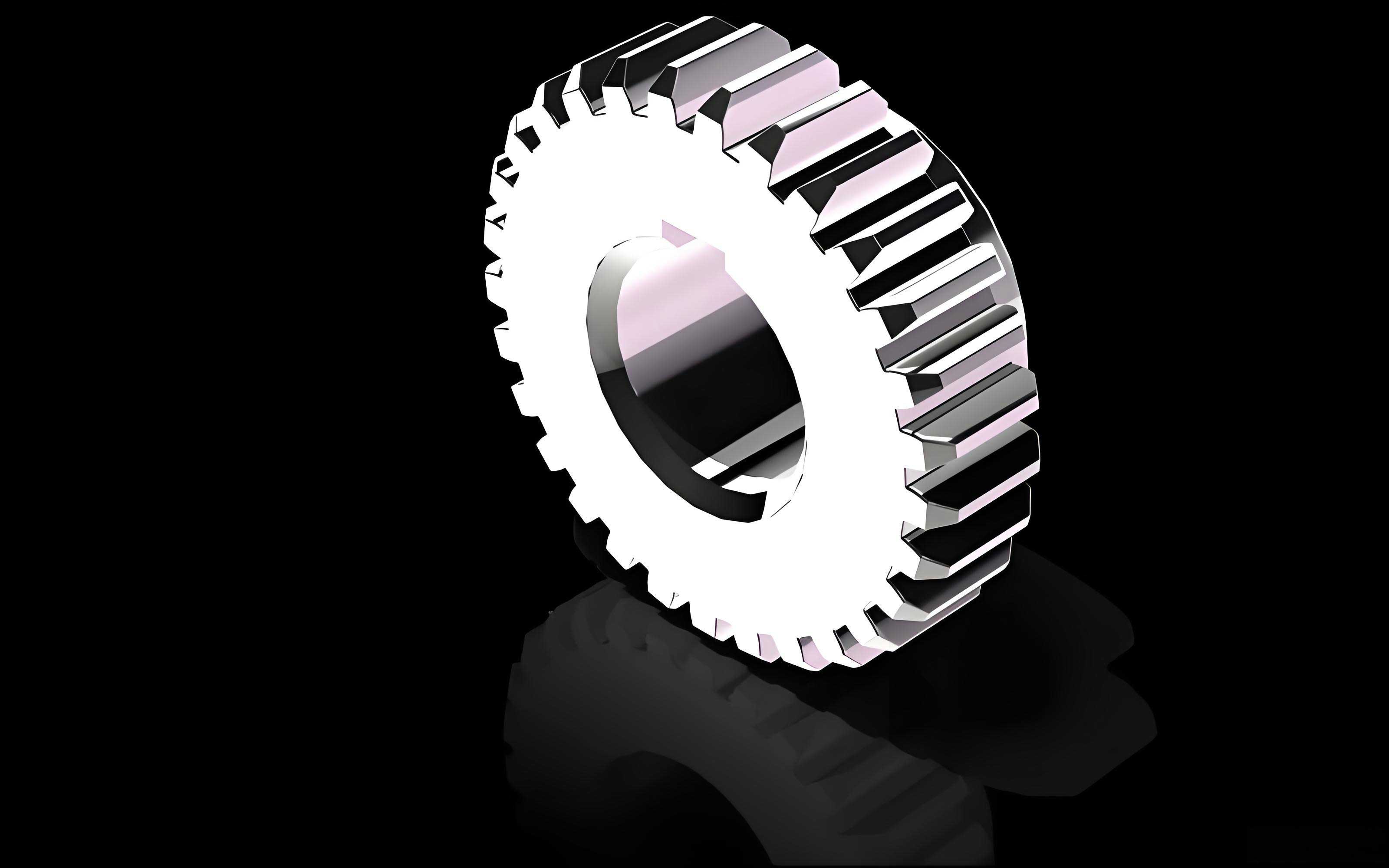
Moving to virtual assembly, the goal is to simulate the meshing of two spur gears with controlled backlash in CATIA’s Assembly Design module. Proper assembly ensures that the spur gears operate smoothly without interference, and it validates the design before physical prototyping. Based on my work, I have identified three precise methods for virtual assembly of spur gears, all relying on constraints that enforce tangency at the pitch circles. These methods address the limitation of generic constraints like contact or coincidence, which may not guarantee accurate meshing for spur gears.
The principle behind virtual assembly for spur gears is to align the gears such that their pitch circles are tangent, maintaining the specified center distance and operating pressure angle. In CATIA, this can be achieved by creating reference geometry—such as planes tangent to the pitch circles and normal planes perpendicular to these tangents—and then applying constraints between them. Table 2 compares the three methods I have developed, each offering a different balance of simplicity and robustness for spur gear assembly.
| Method | Steps | Advantages | Applications |
|---|---|---|---|
| Method 1: Dual Plane Offset | 1. Create tangent and normal planes at pitch circles for both spur gears. 2. Apply offset constraints with zero distance between tangent planes and between normal planes. |
Ensures exact tangency and center distance; robust for dynamic simulation. | Ideal for precise spur gear pairs in critical transmissions. |
| Method 2: Single Plane with Axis Offset | 1. Create tangent or normal planes at pitch circles. 2. Apply offset constraint (zero distance) between planes, and another offset constraint for center distance between gear axes. |
Simpler setup; useful when center distance is explicitly known. | Suitable for spur gear assemblies with fixed center distances. |
| Method 3: Hybrid Approach | 1. Use a combination of tangent and normal planes based on design intent. 2. Apply constraints sequentially to avoid over-constraint. |
Flexible; allows customization for complex spur gear systems. | Best for assemblies with multiple spur gears or non-standard configurations. |
In Method 1, I create a tangent plane at the pitch circle of each spur gear, ensuring it is tangential to the tooth surface at that point. Additionally, I generate a normal plane perpendicular to the tangent plane. For the assembly, I constrain the tangent planes of both spur gears to be offset by zero distance, and similarly for the normal planes. This fully constrains the gears in a way that maintains the correct meshing position, as shown in the assembly diagram. Method 2 is a variation where I use only one set of planes (either tangent or normal) and add an offset constraint for the center distance between the gear axes. For example, with a center distance of 230 mm, I set the axis offset to this value while keeping the plane offset at zero. Method 3 involves a more adaptive approach, selecting planes based on the specific spur gear geometry and applying constraints stepwise to achieve the desired assembly. All these methods leverage CATIA’s bottom-up or top-down assembly capabilities, allowing for associative updates if gear parameters change.
To illustrate, consider a spur gear pair with \(z_1 = 16\), \(z_2 = 29\), \(m = 5\,\text{mm}\), \(\alpha = 20^\circ\), \(x_1 = 0.32\), and \(a’ = 230\,\text{mm}\). After modeling both spur gears as described, I assemble them using Method 1. The result is a virtual spur gear mechanism that can be animated to check for interference and backlash. This process is crucial for validating designs, especially when modification coefficients alter the tooth profiles. By simulating meshing, I can ensure that the spur gears operate without collision and with the intended clearance, which is vital for noise reduction and efficiency in real-world applications.
Beyond basic assembly, CATIA allows for motion analysis through the DMU Kinematics module. Once the spur gears are assembled with proper constraints, I can define a revolute joint for each gear and a gear joint to relate their rotations. The gear ratio is automatically derived from the tooth numbers, enabling dynamic simulation of the spur gear transmission. This virtual prototyping step saves significant time and cost by identifying issues early in the design phase. For instance, I can analyze the contact patterns between teeth to optimize the modification coefficients for load distribution. This holistic approach—from parameterized modeling to virtual assembly and simulation—underscores the power of CATIA for spur gear design.
In my experience, the accuracy of spur gear models directly influences downstream processes like finite element analysis (FEA) and manufacturing. A precise 3D model ensures that stress calculations in FEA reflect real-world conditions, leading to more reliable spur gear designs. Moreover, when exporting models to CNC machines for production, geometric fidelity minimizes errors in tooth cutting. The parameterized method I have described facilitates rapid iteration; for example, if a spur gear pair requires a different center distance, I simply update \(a’\) in CATIA, and all related parameters and the assembly adjust accordingly. This adaptability is key in modern engineering, where customization is common.
To further elaborate on the mathematical aspects, let’s delve into the derivations for modified spur gears. The fundamental equation for the operating pressure angle \(\alpha’\) comes from the geometry of meshing spur gears. Given the actual center distance \(a’\), we have:
$$ a’ = r’_1 + r’_2 = \frac{d’_1 + d’_2}{2} $$
where \(r’_1\) and \(r’_2\) are the operating pitch radii. From the relation between base circles and involute geometry, we know that:
$$ r_b = r \cos \alpha = r’ \cos \alpha’ $$
for each spur gear, with \(r\) as the standard pitch radius. Combining these yields the formula for \(\alpha’\). The total modification coefficient \(x_{\sum}\) is derived from the condition that the sum of tooth thicknesses on the pitch circles equals the circular pitch for proper meshing. This involves the involute function, defined as \(\text{inv}(\alpha) = \tan \alpha – \alpha\). For a spur gear pair, the equation is:
$$ \text{inv}(\alpha’) = \text{inv}(\alpha) + \frac{2(x_1 + x_2) \tan \alpha}{z_1 + z_2} $$
which can be rearranged to solve for \(x_{\sum}\). These formulas are embedded in CATIA’s parameter system, ensuring that the spur gear model adheres to geometric constraints. For clarity, I present Table 3, which lists key formulas used in parameterized modeling of spur gears.
| Formula Name | Equation | Purpose in Spur Gear Modeling |
|---|---|---|
| Operating Pressure Angle | \( \cos \alpha’ = \frac{a}{a’} \cos \alpha \) | Determine meshing angle for given center distance |
| Pitch Circle Diameter | \( d’ = d \frac{\cos \alpha}{\cos \alpha’} \) | Compute diameter at meshing point for each spur gear |
| Center Distance Coefficient | \( y = \frac{z_1 + z_2}{2} \left( \frac{\cos \alpha}{\cos \alpha’} – 1 \right) \) | Account for change in center distance due to modification |
| Total Modification Coefficient | \( x_{\sum} = \frac{z_1 + z_2}{2 \tan \alpha} (\tan \alpha’ – \alpha’ – \tan \alpha + \alpha) \) | Calculate sum of modification coefficients for spur gear pair |
| Tooth Height Modification | \( \Delta y = x_{\sum} – y \) | Adjust addendum to maintain clearance in modified spur gears |
| Addendum Circle Diameter | \( d_a = d + 2(h_a^* + x – \Delta y)m \) | Define outer diameter of modified spur gear |
| Dedendum Circle Diameter | \( d_f = d + 2(h_a^* + c^* – x)m \) | Define root diameter of modified spur gear |
| Involute Cartesian Coordinates | \( x = r_b (\cos \theta + \theta \sin \theta), y = r_b (\sin \theta – \theta \cos \theta) \) | Generate tooth profile curve for spur gear in CATIA |
Implementing these in CATIA requires careful attention to units and angular measures. I typically set angles in degrees for input but convert to radians in formulas where necessary, using CATIA’s built-in functions. For example, to compute \(\alpha’\), I might use a relation like: \(\alpha’ = \arccos\left( \frac{a}{a’} \cos(\alpha \cdot \pi / 180) \right) \cdot 180 / \pi\). This ensures consistency across the spur gear model. Additionally, the parameterized approach allows for scalability; I can easily adapt the process to different types of spur gears, such as those with helical teeth or non-standard profiles, by extending the formulas.
Regarding virtual assembly, the three methods I described can be enhanced with CATIA’s scripting capabilities for automation. Using Visual Basic or CATScript, I can create macros that automatically generate the tangent and normal planes based on spur gear parameters, then apply constraints for assembly. This is particularly useful when dealing with large gear trains involving multiple spur gears. The automation reduces manual effort and minimizes errors, ensuring that each spur gear pair is assembled correctly. Furthermore, I can integrate checks for interference and backlash directly into the script, providing immediate feedback on design viability.
In conclusion, the integration of parameterized modeling and virtual assembly for involute spur gears in CATIA represents a significant advancement in mechanical design. My work demonstrates that by leveraging CATIA’s parametric tools and assembly constraints, engineers can create precise 3D models of modified spur gears and simulate their meshing with accuracy. This approach improves the design, manufacturing, and assembly processes, leading to higher-quality spur gear products. The frequent mention of “spur gear” throughout this article underscores its importance in transmission systems, and the use of tables and formulas aims to provide a clear, actionable reference. As CAD software evolves, techniques like these will become increasingly vital for innovation in gear technology, enabling more efficient and reliable machinery across industries.
To expand on this, let’s consider future directions. With the rise of digital twins and Industry 4.0, the ability to simulate spur gear performance in real-time based on parametric models will be crucial. CATIA’s integration with simulation platforms like SIMULIA allows for coupled analyses, where gear meshing dynamics inform design adjustments. Additionally, additive manufacturing of spur gears benefits from accurate 3D models, as complex geometries can be printed directly from CATIA files. By continuing to refine these methods, we can push the boundaries of spur gear design, achieving optimal performance in diverse applications. I encourage engineers to explore these techniques and contribute to the ongoing development of tools for spur gear innovation.