
I have devoted significant effort to developing parametric drawing techniques specifically tailored for generating detailed working drawings of worm gears that meet industrial production standards. The complexity of worm gears — involving helical threads, meshing profiles, and intricate dimensional relationships — necessitates a systematic approach to automate the drafting process. In this article, I present the key technical solutions I employed, which are equally applicable to other machine parts. The discussion covers the flowchart of parametric drawing, the supporting software environment, and a series of practical techniques to ensure accuracy, stability, and efficiency in dimensioning and graphical construction.
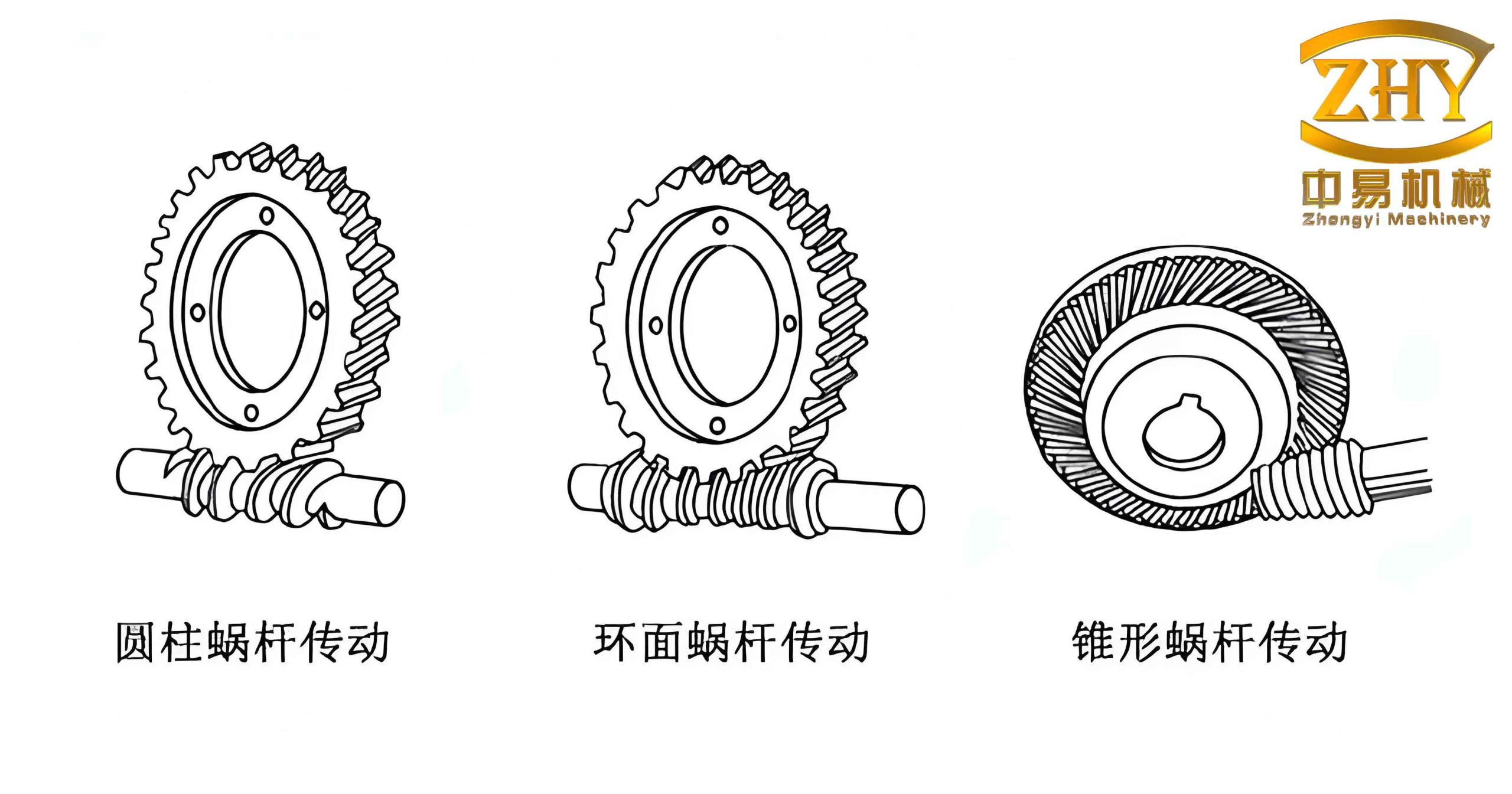
Parametric Drawing Workflow for Worm Gears
The core of my system is a well‑defined sequence of operations that transforms input parameters (module, number of starts, pressure angle, etc.) into a complete working drawing. The flowchart is summarised in the table below, which also indicates the main computational tasks at each stage.
| Step | Activity | Key Data Handled |
|---|---|---|
| 1 | Read input parameters for worm and worm gear | Module \(m\), number of starts \(z_1\), number of teeth \(z_2\), pressure angle \(\alpha\), centre distance \(a\) |
| 2 | Compute basic geometric dimensions | Pitch diameters \(d_{w1}=m z_1 / \tan\gamma\), \(d_{w2}=m z_2\); lead angle \(\gamma\); addendum, dedendum, etc. |
| 3 | Calculate coordinates of key points | Profile points, thread start/end, chamfers, fillets |
| 4 | Load point data into arrays | Structured as \((x, y)\) lists for later plotting |
| 5 | Call parametric drawing subroutines | Line, arc, dimension, hatching commands |
| 6 | Build drawing data file | Instruction set for the graphics kernel |
| 7 | Write instructions and data to a command file | Text‑based or binary intermediate file |
| 8 | Invoke the graphics driver package | Read command file and produce final plot |
The entire process is automated once the user supplies the required parameters. The difficulty lies in handling the variability of dimensions: as the input changes, the positions of dimensions, leaders, and notes must adapt without overlapping or becoming ambiguous.
Supporting Software for Parametric Drawing
My implementation relies on two layers of software: a general‑purpose graphics processing package (referred to as the graphics kernel) and a specialised parametric drawing package that I developed as an interface between the user’s FORTRAN (or C) program and the kernel. The parametric drawing package consists of a set of subroutines that encapsulate common drafting actions — drawing lines, arcs, dimensions, hatching, and text — and automatically adjust to parameter changes. This approach frees the programmer from having to write low‑level graphics instructions for each new part.
Key Parametric Drawing Techniques
Because worm gear drawings contain numerous dimensions, notes, and special symbols (e.g., lead angle, root fillet radii), I had to address several challenges. Below I detail the techniques I adopted.
Maintaining Stable Dimension Positions
Dimensions must remain well‑distributed even when the part geometry changes greatly. My solution is to define all dimension locations relative to a common reference base. For example, in a worm shaft drawing, the axial dimensions of the threaded portion, the plain sections, and the chamfers are all anchored to the left end face of the worm. This base is given a fixed coordinate in the drawing space. As the worm’s length changes, the dimensions shift as a group, preserving their relative spacing.
Let the reference base be point \(B(x_b, y_b)\). For any dimension line that should appear at a distance \(d\) from the base, the coordinate of the dimension line’s start point is
\[
x_{\text{dim}} = x_b + d, \quad y_{\text{dim}} = y_b + \text{offset}
\]
where the offset is a function of the dimension value itself (to avoid text overlap). By recalculating all such positions using the same base, I ensure that the layout remains visually balanced.
Accurate Placement of Dimension Text
The graphics kernel provides a subroutine DIMENSION that draws a dimension line between two measured points and inserts the value. However, this default subroutine often places the text in a location that becomes inappropriate when the part is resized. To overcome this, I use a two‑step approach:
- First, call the kernel’s dimensioning subroutine to draw the lines and arrows.
- Then, erase the automatically placed text and rewrite it at a user‑specified position using a text‑placement subroutine
PLACETEXT.
The parameters of the kernel’s dimensioning subroutine are summarised in the table below.
| Parameter | Description |
|---|---|
| \((x_1, y_1)\) | Start point of the first extension line |
| \((x_2, y_2)\) | Start point of the second extension line |
| \((x_3, y_3)\) | Point on the dimension line (determines its vertical/horizontal position) |
value |
Variable identifier containing the dimension value |
ndec |
Number of decimal places to display |
prefix_control |
0 = no prefix; 1 = prefix “ϕ” (diameter symbol); 2 = prefix “R” (radius); etc. |
tol_low |
Lower deviation (tolerance) |
tol_high |
Upper deviation |
After drawing the dimension lines, I call the kernel’s erase function that removes the last drawn entity. Then I invoke PLACETEXT with the following parameters:
| Parameter | Description |
|---|---|
| \((x_p, y_p)\) | Position where the text is placed |
coord_sys |
0 = absolute coordinates; 1 = relative coordinates |
height |
Character height |
angle |
Rotation angle of the text (degrees) |
justification |
0 = text starts at \((x_p, y_p)\); 1 = text centred on \((x_p, y_p)\); 2 = text ends at \((x_p, y_p)\) |
string |
Character string to display (may include tolerance and prefix) |
For example, to place a diameter dimension \(\phi 100 \pm 0.05\) at a specific location, I first call the kernel’s dimension subroutine (which draws the lines and arrows), then erase the automatically generated text, and finally call PLACETEXT with the string "ϕ100±0.05". The program sequence looks like:
CALL DIMENSION(X1,Y1,X2,Y2,X3,Y3, VALUE, 2, 1, -0.05, 0.05)
CALL ERASE_LAST_ENTITY
CALL PLACETEXT(XP,YP, 0, 3.5, 0.0, 1, "ϕ100±0.05")
Angle Dimensioning Between Two Lines
Worm gears often require angular dimensions — for example, the lead angle \(\gamma\) or the chamfer angle. The kernel provides a subroutine ANGLE_DIM that draws an arc and places the degree, minute, and second values. However, it cannot display tolerances such as “\(30^\circ \pm 10’\)”. I therefore use the same erase‑and‑rewrite technique.
| Parameter | Description |
|---|---|
| \((x_1, y_1)\), \((x_2, y_2)\) | Two points on the first line |
| \((x_3, y_3)\), \((x_4, y_4)\) | Two points on the second line |
| \((x_r, y_r)\) | Location of the dimension arc (controls radius) |
| \((x_s, y_s)\) | Start point of the angle text |
deg, min, sec |
Actual angle in degrees, minutes, seconds (real numbers) |
After the arc and arrow are drawn, I erase the original text and call PLACETEXT to write a formatted string such as “\(30^\circ \pm 10’\)”. The FORMAT statement in FORTRAN can produce the degree symbol using an appropriate character code. For example:
CALL ANGLE_DIM( ... , 30.0, 0.0, 0.0)
CALL ERASE_LAST_ENTITY
WRITE(STRING, 100) DEG, MIN, SEC
100 FORMAT(F4.1,'°±',F4.1,'\'')
CALL PLACETEXT(XT, YT, 0, 3.5, 0.0, 0, STRING)
Drawing Arrowheads for Radii and Diameters
Many worm gear features — such as root fillet radii and shaft shoulder diameters — require a leader line with an arrowhead. I created a dedicated subroutine ARROW that draws a filled arrowhead between two points.
| Parameter | Description |
|---|---|
| \((x_{\text{head}}, y_{\text{head}})\) | Arrow tip coordinate |
| \((x_{\text{tail}}, y_{\text{tail}})\) | Arrow tail coordinate (where the leader line ends) |
org_x, org_y |
Origin of the current coordinate system (used for scaling the arrow size) |
For example, to label a cylindrical diameter of a worm gear blank, I first draw the leader line from the feature to a note point, then call ARROW with the tip at the feature edge. The associated text (e.g., “\(\phi 80\)”) is placed using PLACETEXT.
CALL LINE( ... )    ! draw leader
CALL ARROW(XTIP, YTIP, XLEADER, YLEADER, 0.0, 0.0)
CALL PLACETEXT(XNOTE, YNOTE, 0, 3.5, 0.0, 0, "ϕ80")
Block Handling for Complex Hatched Regions
One of the most time‑consuming tasks in worm gear drawings is hatching the cross‑sectional areas. The parametric package includes two subroutines for managing blocks: BLOCK_SAVE and BLOCK_INSERT. Using these, I can draw a complex region once, define it as a block, and then insert it repeatedly after applying hatching only to the block contents.
| Subroutine | Parameter | Description |
|---|---|---|
BLOCK_SAVE |
\((x_{\text{base}}, y_{\text{base}})\) | Base point for the block (reference for insertion) |
| \((x_{\text{win1}}, y_{\text{win1}})\), \((x_{\text{win2}}, y_{\text{win2}})\) | Window corners defining the entities to include | |
block_name |
An 8‑character name for the block | |
BLOCK_INSERT |
block_name |
Name of the previously saved block |
| \((x_{\text{ins}}, y_{\text{ins}})\) | Insertion point (block base point aligns with this) | |
scale_x, scale_y |
Scaling factors (typically 1.0) | |
rotation |
Rotation angle in degrees |
A typical use case is hatching the tooth space of a worm wheel. I first draw the closed outline of the space, call the kernel’s hatching command, then save the hatched area as a block. Later, when drawing the full wheel, I can insert this block at every tooth space position, saving repeated hatching calculations. The following example draws a square with a circle inside, hatches the region between them, saves it as a block, then draws a second circle and hatches it, and finally inserts the original block to create a complex assembly.
CALL PLACE_ORIGIN(0.0, 0.0)
CALL LINETYPE(0)                     ! solid line
! Draw square from (0,0) to (10,10)
CALL RECTANGLE(0.0, 0.0, 10.0, 10.0)
! Draw circle centre (5,5) radius 2
CALL CIRCLE(5.0, 5.0, 2.0)
! Hatch between square and circle
CALL HATCH_REGION( ... )
! Save block named 'BLK1'
CALL BLOCK_SAVE(5.0,5.0, 0.0,0.0, 10.0,10.0, 'BLK1')
! Now draw a new circle centre (15,15) radius 3
CALL CIRCLE(15.0, 15.0, 3.0)
! Hatch that circle (internal hatching)
CALL HATCH_CIRCLE(15.0, 15.0, 3.0)
! Insert block BLK1 at (15,15) (will place the square+circle pattern)
CALL BLOCK_INSERT('BLK1', 15.0, 15.0, 1.0, 1.0, 0.0)
! Draw centre line
CALL LINETYPE(2)
CALL LINE(0.0,5.0, 20.0,5.0)
By using block insertion, I eliminated the need to recalculate hatching boundaries for repeated features — a critical speed‑up for worm gear drawings with many identical tooth profiles.
Application to Worm Gear Drawing Software
I combined these techniques into a comprehensive parametric drawing system for worm gears. The system accepts inputs such as the module, number of starts of the worm, number of teeth of the worm gear, pressure angle, and centre distance. It then computes all necessary dimensions, generates the worm shaft drawing (including thread profile, chamfers, keyways) and the worm gear wheel drawing (including tooth space profiles, hub, rim). The dimensioning is automatically placed according to the stable‑base principle, and all special symbols (lead angle, diameter prefixes, tolerances) are inserted using the erase‑and‑rewrite method. Arrowheads are drawn with the dedicated subroutine, and hatching of tooth spaces is expedited by block handling.
The software successfully produces production‑ready working drawings that comply with industry standards. It handles multiple worm gear types (single‑start, multi‑start, right‑hand, left‑hand) without user intervention beyond the initial parameters.
Conclusion
The parametric drawing techniques I developed for worm gears are not restricted to this single component. The principles — stable reference‑based dimensioning, text repositioning, angle notation with tolerances, custom arrowhead subroutines, and block handling for hatching — are universally applicable to parametric drafting of machine parts. They significantly reduce the coding effort for new components while ensuring that the resulting drawings remain clear and accurate regardless of parameter variation. I believe these methods offer a practical foundation for building flexible CAD systems in small and medium‑sized manufacturing enterprises.