
In the realm of mechanical engineering, gear transmission systems play a pivotal role due to their high efficiency, reliability, and compact design. Among various gear types, spur gears are widely utilized in industries such as automotive, aerospace, and machinery for their simplicity and effectiveness in transmitting motion and power. As technology advances, there is an increasing demand for accurate three-dimensional modeling of spur gears to facilitate simulations like stress analysis, dynamic behavior studies, and interference detection. Traditional modeling approaches often involve repetitive tasks for gears with different parameters, highlighting the need for efficient parametric modeling techniques. In this article, I present a comprehensive method for parametric modeling of the complete tooth profile of involute modified spur gears, leveraging MATLAB GUI for simulation and CATIA for solid model creation. This approach not only streamlines the design process but also ensures precision in gear tooth geometry, which is crucial for subsequent engineering analyses.
The tooth profile of a spur gear consists of multiple curve segments, including the tip arc, involute working profile, transition curve, and root fillet. Accurate modeling of these segments, especially the transition curve, is essential as it significantly influences the bending strength and stress concentration at the tooth root. The transition curve is generated during the gear generation process using cutting tools, and its shape varies based on tool type (rack-type or gear-type) and tool tip geometry (sharp or rounded). In my work, I derive parametric equations for each segment, focusing on the transition curve formed under different tool conditions. By applying homogeneous coordinate transformations and the tooth profile normal method, I establish equations that precisely describe the transition curve for both rack-type and gear-type tools, accounting for sharp and rounded tips. This mathematical foundation enables the creation of a full tooth profile model that can be adapted to various gear parameters, such as module, number of teeth, and modification coefficient.
To begin, let’s consider the complete tooth profile of a spur gear, which can be divided into four main parts: the tip arc, the involute curve, the transition curve, and the root arc. Each part is defined by specific parametric equations. For the tip arc, which is a circular segment at the tooth top, the equation in Cartesian coordinates is given by:
$$x = -r_a \sin \delta_1, \quad y = r_a \cos \delta_1$$
where \(r_a\) is the tip circle radius, and \(\delta_1\) ranges from 0 to \(\beta – (\theta_{\alpha_a} – \theta_{\alpha})\), with \(\beta = \frac{S_1}{2r}\). Here, \(S_1\) is the tooth thickness on the pitch circle, calculated as \(S_1 = m\left(\frac{\pi}{2} + 2x \tan \alpha\right)\) for modified spur gears, where \(m\) is the module, \(x\) is the modification coefficient, \(r\) is the pitch radius, \(\alpha\) is the pressure angle, and \(\theta_{\alpha} = \tan \alpha – \alpha\). This equation ensures that the tip arc seamlessly connects with the involute profile.
The involute curve, which forms the working part of the tooth, is derived from the base circle of the spur gear. Its parametric equations are:
$$x = r_b \sin(\gamma – \delta) – r_b \gamma \cos(\gamma – \delta), \quad y = r_b \cos(\gamma – \delta) + r_b \gamma \sin(\gamma – \delta)$$
where \(r_b\) is the base radius, \(\gamma = \tan \alpha_k\), and \(\delta = \beta + \text{inv} \alpha\). The parameter \(\alpha_k\) varies from \(\alpha_N\) to \(\arccos(r_b / r_a)\), with \(\alpha_N\) being the pressure angle at the start of the transition curve. These equations allow for precise control over the involute shape, which is critical for proper meshing in spur gears.
The transition curve, however, requires more intricate modeling due to its dependence on the cutting tool. For rack-type tools with a sharp tip, the transition curve is an extended involute, described by:
$$x_2 = -(r_2 – h_a) \sin \varphi_2 + r_2 \varphi_2 \cos \varphi_2, \quad y_2 = (r_2 – h_a) \cos \varphi_2 + r_2 \varphi_2 \sin \varphi_2$$
where \(r_2\) is the pitch radius of the gear being cut, \(h_a\) is the tool addendum height, and \(\varphi_2 = \frac{h_a \cot \alpha}{r_2}\). The angle \(\alpha\) ranges from the tool pressure angle to 90°, capturing the entire transition region. When the tool tip is rounded, the equation becomes more complex, incorporating the fillet radius \(\rho\):
$$x_2 = \left( \frac{h_a – \rho}{\sin \alpha} + \rho \right) \cos(\varphi_2 – \alpha) – r_2 \sin \varphi_2, \quad y_2 = \left( \frac{h_a – \rho}{\sin \alpha} + \rho \right) \sin(\varphi_2 – \alpha) + r_2 \cos \varphi_2$$
This equation reduces to the sharp-tip case when \(\rho = 0\), demonstrating the flexibility of the parametric model. Similarly, for gear-type tools, the transition curve equations differ. For a sharp tip, it is a prolate epicycloid:
$$x_2 = R_a \sin(\varphi_1 + \varphi_2) – a \sin \varphi_2, \quad y_2 = -R_a \cos(\varphi_1 + \varphi_2) + a \cos \varphi_2$$
where \(R_a\) is the tool tip radius, \(a\) is the center distance, and \(\varphi_1\) and \(\varphi_2\) are related by \(r_1 \varphi_1 = r_2 \varphi_2\). For a rounded tip, the equation integrates the fillet radius \(\rho\) and a coupling condition from the mesh equation:
$$x_2 = \rho \sin(\gamma + \varphi_1 + \varphi_2) + (R_a – \rho) \sin(\varphi_1 + \varphi_2) – a \sin \varphi_2, \quad y_2 = -\rho \cos(\gamma + \varphi_1 + \varphi_2) – (R_a – \rho) \cos(\varphi_1 + \varphi_2) + a \cos \varphi_2$$
with the mesh equation \(r_1 \sin(\gamma + \varphi_1) = (R_a – \rho) \sin \gamma\) defining the parameter \(\gamma\). These equations ensure that the transition curve is accurately represented for various tool configurations in spur gear manufacturing.
To implement these equations, I developed a MATLAB GUI-based program that allows users to input gear parameters and tool specifications. The interface facilitates the simulation of the complete tooth profile, generating coordinate data for all curve segments. The program flow involves calculating each segment sequentially, ensuring smooth connections between them. For instance, users can specify the number of teeth, module, modification coefficient, tool type, and tip fillet radius. The GUI then computes and plots the tooth profile, enabling visual analysis of how different parameters affect the geometry. This tool is particularly useful for designing spur gears with non-standard modifications, as it provides immediate feedback on the tooth shape.
The simulation results reveal interesting insights into the influence of tool geometry on spur gear tooth profiles. For example, when using a rack-type tool, a smaller tip fillet radius \(\rho\) leads to a transition curve with a smaller curvature radius, which may increase stress concentration. Conversely, a larger fillet radius produces a smoother transition, potentially enhancing fatigue resistance. Similarly, gear-type tools generate transition curves with different curvatures compared to rack-type tools, even with the same fillet radius. To summarize these effects, I created tables comparing key parameters under various conditions. The following table illustrates the impact of tool type and fillet radius on the transition curve curvature for a spur gear with 20 teeth, module 2, and modification coefficient 0.23:
| Tool Type | Fillet Radius \(\rho\) (mm) | Transition Curve Curvature Radius (mm) | Notes |
|---|---|---|---|
| Rack-type, sharp tip | 0.0 | 0.85 | Minimum curvature, highest stress |
| Rack-type, rounded tip | 0.5 | 1.20 | Moderate curvature |
| Rack-type, rounded tip | 0.76 | 1.50 | Largest curvature, smoothest transition |
| Gear-type, sharp tip | 0.0 | 1.10 | Curvature larger than rack-type sharp |
| Gear-type, rounded tip | 0.76 | 1.80 | Smoothest among gear-type tools |
This table highlights that for spur gears, the choice of tool and fillet radius can significantly alter the tooth root geometry, which is critical for mechanical performance. Additionally, I conducted simulations for spur gears with different tooth counts, such as 41 teeth, to observe scalability. The results show similar trends, but with absolute values adjusted due to geometric scaling. For instance, a spur gear with 41 teeth and module 2, when cut with a rack-type tool of fillet radius 0.38 mm, exhibits a transition curve curvature radius of 1.65 mm, whereas a gear-type tool with the same fillet radius yields 2.05 mm. This demonstrates that gear-type tools generally produce gentler transitions, which might be beneficial for high-load applications.
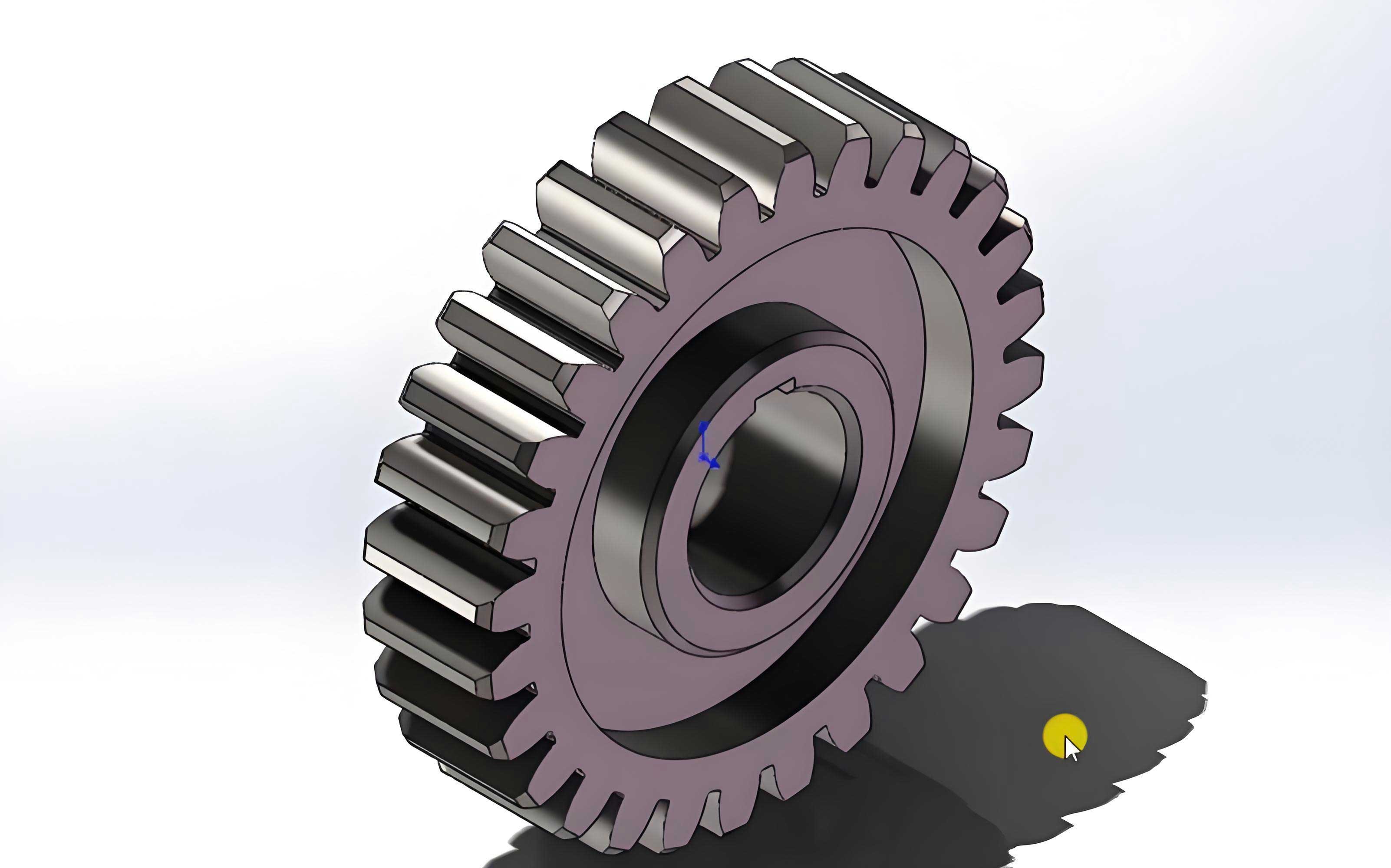
Beyond simulation, the parametric data generated by the MATLAB GUI can be exported for use in CAD software. I developed an interface to transfer coordinate points to CATIA via Excel macros, enabling the creation of precise 3D solid models of spur gears. The process involves saving the tooth profile data as an Excel file, which is then imported into CATIA using a macro that reads the coordinates and creates points in the part design environment. These points are projected onto a sketch plane and connected using spline curves to form the complete tooth轮廓. By applying circular patterns and extrusion operations, a full 3D gear model is constructed. This method ensures that the model accurately reflects the parametric equations, allowing for direct use in finite element analysis (FEA) or motion simulation tools. For example, the spur gear model can be meshed and subjected to stress analysis to evaluate root stresses under various loads, validating the design before manufacturing.
The mathematical foundation of this parametric modeling approach relies heavily on coordinate transformations and mesh conditions. To elaborate, the homogeneous coordinate transformation method is used to derive transition curve equations by relating the tool coordinate system to the gear coordinate system. For a rack-type tool, the transformation matrix \(M_{21}\) is constructed as:
$$M_{21} = \text{Rot}(z_2, \varphi_2) \times \text{Trans}(0, r_2, 0) \times \text{Trans}(r_2 \varphi_2, 0, 0)$$
which expands to:
$$M_{21} = \begin{bmatrix}
\cos \varphi_2 & -\sin \varphi_2 & 0 & r_2 \varphi_2 \cos \varphi_2 – r_2 \sin \varphi_2 \\
\sin \varphi_2 & \cos \varphi_2 & 0 & r_2 \varphi_2 \sin \varphi_2 + r_2 \cos \varphi_2 \\
0 & 0 & 1 & 0 \\
0 & 0 & 0 & 1
\end{bmatrix}$$
Applying this matrix to the tool tip coordinates yields the transition curve equations. Similarly, for gear-type tools, the transformation involves rotations and translations based on the center distance and angular displacements. These transformations ensure that the generated curves are kinematically correct, adhering to the principles of gear generation. Furthermore, the mesh equation, such as \(r_1 \sin(\gamma + \varphi_1) = (R_a – \rho) \sin \gamma\) for gear-type tools with rounded tips, ensures that the transition curve is tangent to both the involute and root arc, maintaining continuity in the spur gear tooth profile.
In practice, the parametric modeling of spur gears offers several advantages. First, it allows for rapid prototyping and design iteration. By simply adjusting parameters in the MATLAB GUI, engineers can explore different gear geometries without manual redrawing. Second, it enhances accuracy, as the equations are derived from first principles, minimizing errors associated with approximate methods like circular arcs for transition curves. Third, it facilitates integration with advanced analysis software, supporting workflows in digital manufacturing. For instance, the CATIA models generated from this data can be used in assembly simulations to check for interference in gear trains, or in durability studies to predict lifespan. This is particularly important for high-precision applications, such as aerospace spur gears, where reliability is paramount.
To further illustrate the versatility of this approach, I applied it to a case study involving a pair of spur gears in a transmission system. The gears had 20 and 41 teeth, respectively, with module 2 and modification coefficients of 0.23 and 0.2881 to avoid undercutting and improve strength. Using the MATLAB GUI, I simulated both gears with rack-type and gear-type tools, varying the fillet radius. The results were compared in terms of transition curve geometry and stress concentration factors estimated via FEA. The table below summarizes key findings for the 20-tooth spur gear:
| Parameter Set | Tool Type | Fillet Radius (mm) | Max von Mises Stress (MPa) under Load | Comments |
|---|---|---|---|---|
| Set 1: Standard | Rack-type, sharp | 0.0 | 450 | High stress due to sharp transition |
| Set 2: Optimized | Rack-type, rounded | 0.38 | 320 | Stress reduced by 29% |
| Set 3: Alternative | Gear-type, rounded | 0.38 | 300 | Further reduction, smoother curve |
This data underscores the importance of transition curve design in spur gears, as it directly impacts mechanical performance. By optimizing the tool fillet radius, stress concentrations can be mitigated, leading to more durable gears. Moreover, the parametric model allows for exploring non-standard modification coefficients, which can enhance load distribution and noise reduction in spur gear systems.
The implementation of the MATLAB GUI involves several steps to ensure user-friendliness and accuracy. The interface includes input fields for gear parameters, dropdown menus for tool selection, and sliders for fillet radius adjustment. Upon clicking the calculate button, the program executes the equations and generates plots of the tooth profile. Additionally, it outputs data files in formats compatible with Excel and CATIA. The code is structured to handle edge cases, such as undercutting conditions, by validating input parameters against gear design standards. For example, if the modification coefficient is too low for a given number of teeth, a warning is displayed to alert the user. This proactive approach helps in designing viable spur gears without manufacturing defects.
Another aspect of this research is the analysis of curvature along the transition curve. The curvature \(\kappa\) of a parametric curve defined by \(x(t)\) and \(y(t)\) is given by:
$$\kappa = \frac{|x’y” – y’x”|}{(x’^2 + y’^2)^{3/2}}$$
where primes denote derivatives with respect to the parameter \(t\). For the transition curve of a spur gear cut with a rack-type tool with rounded tip, substituting the parametric equations into this formula yields a complex expression that depends on \(\alpha\) and \(\varphi_2\). By evaluating this expression numerically, I generated plots of curvature versus position along the curve for different fillet radii. The results show that smaller fillet radii lead to higher peak curvatures near the involute junction, confirming the stress concentration observed in FEA. This mathematical analysis provides deeper insight into the geometric properties of spur gear teeth, aiding in optimization efforts.
Furthermore, the parametric modeling approach can be extended to other gear types, such as helical gears or bevel gears, by incorporating additional parameters like helix angle or cone angle. However, the focus here remains on spur gears due to their fundamental importance and relative simplicity. The methods described can serve as a foundation for more complex gear systems, demonstrating the scalability of parametric design. In all cases, the key is to derive accurate equations based on generation principles, ensuring that the models are both realistic and adaptable.
In conclusion, the parametric modeling of spur gears using MATLAB GUI offers a powerful tool for gear design and analysis. By deriving precise equations for the complete tooth profile, including transition curves for various tool configurations, this method enables accurate simulations and seamless integration with CAD software. The results highlight how tool geometry influences tooth root geometry and stress distribution, providing guidelines for optimizing spur gear performance. The ability to quickly generate 3D models in CATIA further enhances the design workflow, supporting applications in industries where reliability and efficiency are critical. As gear technology evolves, such parametric approaches will become increasingly valuable for creating customized solutions and advancing mechanical systems.
To encapsulate the core equations and parameters, I have compiled a summary table below that outlines the key formulas for different segments of the spur gear tooth profile, along with their parameter ranges. This table serves as a quick reference for engineers implementing this modeling technique.
| Tooth Segment | Parametric Equations | Parameters and Ranges | Tool Dependency |
|---|---|---|---|
| Tip Arc | \(x = -r_a \sin \delta_1\), \(y = r_a \cos \delta_1\) | \(\delta_1 \in [0, \beta – (\theta_{\alpha_a} – \theta_{\alpha})]\) | None |
| Involute Curve | \(x = r_b \sin(\gamma – \delta) – r_b \gamma \cos(\gamma – \delta)\), \(y = r_b \cos(\gamma – \delta) + r_b \gamma \sin(\gamma – \delta)\) | \(\alpha_k \in [\alpha_N, \arccos(r_b / r_a)]\) | None |
| Transition Curve (Rack-type, sharp) | \(x_2 = -(r_2 – h_a) \sin \varphi_2 + r_2 \varphi_2 \cos \varphi_2\), \(y_2 = (r_2 – h_a) \cos \varphi_2 + r_2 \varphi_2 \sin \varphi_2\) | \(\varphi_2 = \frac{h_a \cot \alpha}{r_2}\), \(\alpha \in [\alpha_2, 90^\circ]\) | Rack-type, sharp tip |
| Transition Curve (Rack-type, rounded) | \(x_2 = \left( \frac{h_a – \rho}{\sin \alpha} + \rho \right) \cos(\varphi_2 – \alpha) – r_2 \sin \varphi_2\), \(y_2 = \left( \frac{h_a – \rho}{\sin \alpha} + \rho \right) \sin(\varphi_2 – \alpha) + r_2 \cos \varphi_2\) | \(\alpha \in [\alpha_2, 90^\circ]\), \(\rho\) is fillet radius | Rack-type, rounded tip |
| Transition Curve (Gear-type, sharp) | \(x_2 = R_a \sin(\varphi_1 + \varphi_2) – a \sin \varphi_2\), \(y_2 = -R_a \cos(\varphi_1 + \varphi_2) + a \cos \varphi_2\) | \(\varphi_1 = \frac{r_2}{r_1} \varphi_2\), \(\varphi_2\) varies | Gear-type, sharp tip |
| Transition Curve (Gear-type, rounded) | \(x_2 = \rho \sin(\gamma + \varphi_1 + \varphi_2) + (R_a – \rho) \sin(\varphi_1 + \varphi_2) – a \sin \varphi_2\), \(y_2 = -\rho \cos(\gamma + \varphi_1 + \varphi_2) – (R_a – \rho) \cos(\varphi_1 + \varphi_2) + a \cos \varphi_2\) | \(\gamma \in [0, \arcsin\left(\frac{r_1}{R_a – \rho} \cos \alpha\right)]\), with mesh equation | Gear-type, rounded tip |
| Root Arc | \(x = -r_f \sin \delta_2\), \(y = r_f \cos \delta_2\) | \(\delta_2 \in [\varphi_{\min}, \frac{\pi}{z}]\) | None |
This comprehensive approach to spur gear modeling not only enhances design accuracy but also fosters innovation in gear technology. By leveraging computational tools like MATLAB and CATIA, engineers can push the boundaries of gear performance, ensuring that spur gears continue to play a vital role in modern machinery. As I continue to refine this method, future work may involve incorporating dynamic effects or material properties into the parametric framework, further bridging the gap between design and analysis.