
1. Introduction
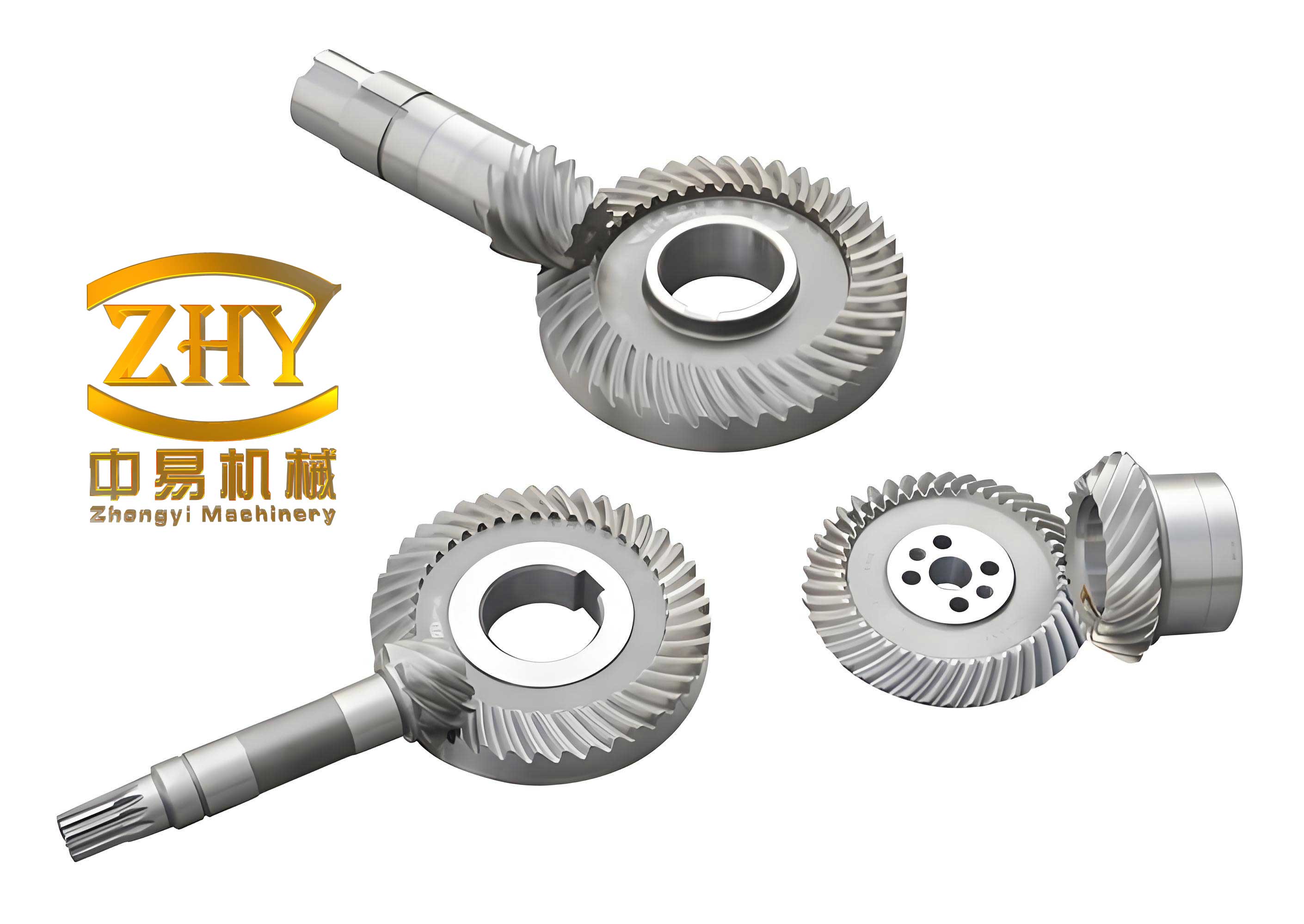
Hypoid gears enable motion and power transmission between intersecting axes, offering advantages such as high load capacity, large contact ratio, smooth transmission, and low noise. Consequently, they are extensively utilized across marine, mechanical, automotive, aerospace, and aviation engineering fields. Hypoid gears are partially conjugated, localized point-contact gear pairs, characterized by complex tooth surface geometry and intricate machine-tool adjustment parameters. As critical components for power transmission, their performance directly impacts the lifespan, reliability, and vibration/noise characteristics of the entire driveline system.
To achieve desired meshing performance, Tooth Contact Analysis (TCA) serves as a vital computer-aided simulation tool. TCA allows for the simulation of gear meshing conditions, including contact patterns and transmission errors, prior to physical manufacturing. This facilitates the adjustment of machining parameters to obtain ideal meshing characteristics, significantly reducing prototyping cycles and production costs. Traditional theoretical TCA methods require solving five non-linear equations to obtain contact points, followed by calculations of principal directions and curvatures at those points. This approach is computationally intensive, sensitive to initial guesses, and less adaptable. In contrast, the Ease-off-TCA method reduces the required equations to two, simplifies the calculation of the contact ellipse major axis by avoiding complex curvature calculations, and offers higher efficiency, simplicity, and precision, particularly for edge contact analysis.
The finite element method (FEM) is increasingly used in engineering. However, traditional gear FEM analysis often involves reconstructing tooth surfaces in CAD software from point clouds, importing into FEM tools, and manually performing assembly and meshing. This process is inefficient, has poor repeatability, and can introduce significant errors. Manual assembly often leads to interference or gaps, compromising analysis accuracy. To overcome these limitations, a new approach is needed for automatic mesh generation and precise model assembly, which this study addresses.
Furthermore, the performance of machined hypoid gears often requires modification. Presently, this is achieved by altering machine-tool settings, such as the ratio-of-roll coefficient, or through complex tooth surface design and reconstruction. This work explores an alternative: modifying the pinion cutter blade design, replacing conventional straight blades with curved blades. This approach offers a more straightforward and feasible method for tooth surface modification and performance improvement.
2. Mathematical Modeling and Cutting Simulation
I established precise mathematical models for both the gear (ring gear) and pinion based on differential geometry and gearing theory. The gear is manufactured using the Formate process, while the pinion is produced using the tilt method. The derivation includes equations for both the working tooth surface and the transition fillet surface.
2.1 Gear Tooth Surface Equation (Formate Process)
For the gear (index 2), the cutter blade is a straight line. The cutting edge surface and normal equations in the cutter coordinate system $S_G$ are given by:
$$ \vec{r}_G(s_G, \theta_G) = \begin{bmatrix} -r_{c2} \cos \alpha_G \\ (r_{c2} – s_G \sin \alpha_G) \sin \theta_G \\ (r_{c2} – s_G \sin \alpha_G) \cos \theta_G \\ 1 \end{bmatrix} $$
$$ \vec{n}_G(\theta_G) = \begin{bmatrix} \sin \alpha_G \\ -\cos \alpha_G \sin \theta_G \\ -\cos \alpha_G \cos \theta_G \end{bmatrix} $$
Where $r_{c2}$ is the cutter tip radius, $\alpha_G$ is the blade pressure angle, and $s_G, \theta_G$ are the surface parameters. By applying coordinate transformations to the fixed gear coordinate system $S_2$, the working surface equation is obtained:
$$ \vec{r}_2(\theta_G, s_G) = [M_{2B}][M_{BG}] \vec{r}_G(s_G, \theta_G) $$
$$ \vec{n}_2(\theta_G) = [L_{2B}][L_{BG}] \vec{n}_G(\theta_G) $$
The transition fillet surface, generated by the cutter tip radius $r_{f2}$, is derived similarly. The boundary line between the working and fillet surfaces is found by setting the fillet parameter $\theta_{f2}$ equal to $\alpha_G$ for the convex side or $\pi – \alpha_G$ for the concave side.
2.2 Pinion Tooth Surface Equation (Tilt Process)
The pinion (index 1) is generated with a complex kinematic relationship. The cutter surface is defined in its own coordinate system $S_P$. The surface and normal equations are:
$$ \vec{r}_P(s_P, \theta_P) = \begin{bmatrix} (r_{c1} + s_P \sin \alpha_P) \cos \theta_P \\ (r_{c1} + s_P \sin \alpha_P) \sin \theta_P \\ -s_P \cos \alpha_P \\ 1 \end{bmatrix} $$
$$ \vec{n}_P(\theta_P) = \begin{bmatrix} \cos \alpha_P \cos \theta_P \\ \cos \alpha_P \sin \theta_P \\ -\sin \alpha_P \end{bmatrix} $$
The transformation from the cutter to the machine coordinate system involves several steps. The pinion generation process is a conjugate motion, governed by the equation of meshing:
$$ f(s_P, \theta_P, \phi_{c1}) = \vec{n}_D \cdot \vec{v}^{(c1)}_D = 0 $$
Here, $\vec{v}^{(c1)}_D$ is the relative velocity vector between the cutter and the workpiece, and $\phi_{c1}$ is the cradle rotation angle. Solving this equation eliminates one parameter (e.g., $s_P$). The final pinion tooth surface is obtained through a series of coordinate transformations $[M]$, mapping the cutter surface to the pinion coordinate system $S_1$:
$$ \vec{r}_1(\theta_P, \phi_{c1}) = [M_{1F}][M_{FE}][M_{ED}][M_{DC}][M_{CA}][M_{AP}] \vec{r}_P(\theta_P, \phi_{c1}) $$
2.3 Tooth Surface Grid Generation and Positioning
For numerical simulation and visualization, I discretized the tooth surfaces into a grid of points defined on the rotary projection plane. As shown below, the grid points are characterized by coordinates $(v_{ij}, h_{ij})$ along the face width and tooth height directions.
| Parameter | Symbol | Formula |
|---|---|---|
| Face width coordinate | $v_{ij}$ | $v_{ij} = A_i + (j-1)(A_o – A_i)/(n-1)$ |
| Tooth height coordinate | $h_{ij}$ | $h_{ij} = H_j + (i-1)(H’_j – H_j)/(m-1)$ |
These grid coordinates are incorporated into the tooth surface equations, forming a system of non-linear equations that I solved using MATLAB’s `fsolve` function. This process yields the precise 3D coordinates for each grid point, enabling the visualization of the complex tooth geometry.
Accurate positioning of the pinion concave and convex flanks is crucial. I utilized the pitch line check dimensions: the mid-point chordal height $h_{m1}$ and the mid-point chordal thickness $s_{n1}$. The positioning angle $\theta_x$ is calculated based on the condition that the distance between the concave flank contact point $O_v$ and the convex flank contact point $O_x$ equals the mid-point chordal thickness:
$$ | \vec{O_v} – \vec{O_x} | = s_{n1} $$
This step ensures the correct tooth thickness and relative flank positions. The accuracy of the derived mathematical models was validated by confirming the continuity between the working and fillet surfaces at their boundary.
2.4 Solid Modeling and Comparison
I developed 3D solid models using two approaches: a “cutting simulation” method within CATIA, which mimics the actual machining process, and a “reverse modeling” method, which fits surfaces to the generated point clouds. A deviation analysis comparing the models against the theoretical point clouds showed the cutting simulation method to be superior.
| Modeling Method | Gear Deviation (mm) | Pinion Deviation (mm) |
|---|---|---|
| Cutting Simulation | 0.007 – 0.065 | 0.000 – 0.030 |
| Reverse Modeling | 0.035 – 0.171 | 0.000 – 0.116 |
The cutting simulation model exhibited significantly lower deviations, confirming its higher precision and validating the mathematical model. The accuracy of this method is dependent on the discretization step (n=80) of the generating motion, with finer steps leading to higher fidelity models.
3. Tooth Contact Analysis (TCA)
3.1 Theoretical TCA
The classical TCA algorithm involves simulating the meshing of the gear and pinion based on their mathematical models. I established the fundamental equations requiring equal position vectors and surface normals in the fixed coordinate system $S_h$. For each increment of the pinion rotation angle $\phi_1$, the other unknown parameter set is solved from:
$$ \begin{cases} \vec{r}^{(1)}_h(\theta_P, \phi_{c1}, \phi_1) = \vec{r}^{(2)}_h(\theta_G, s_G, \phi_2) \\ \vec{n}^{(1)}_h(\theta_P, \phi_{c1}, \phi_1) = \vec{n}^{(2)}_h(\theta_G, s_G, \phi_2) \end{cases} $$
This system, when reduced to scalar form, consists of 5 independent equations. The series of solved contact points traces the contact path on the tooth surface. The instantaneous transmission error $\delta\phi_2$ is computed as the deviation of the actual gear rotation from the theoretical rotation:
$$ \delta\phi_2 = \phi_2 – \phi^{(0)}_2 – \frac{Z_1}{Z_2}(\phi_1 – \phi^{(0)}_1) $$
To determine the contact ellipse dimensions, I calculated the principal curvatures and directions of both surfaces at the contact point. The elastic deformation $\varepsilon$ is assumed to be 0.00635 mm (per Gleason’s practice). The semi-axes $a$ and $b$ of the contact ellipse are calculated from the relative principal curvatures $K_\Sigma$ and $g$:
$$ A = \frac{1}{4}(K^{(1)}_\Sigma + K^{(2)}_\Sigma – \sqrt{g_1^2 + g_2^2 – 2g_1 g_2 \cos 2\sigma}) $$
$$ a = \sqrt{\frac{\varepsilon}{A}}, \quad B = \frac{1}{4}(K^{(1)}_\Sigma + K^{(2)}_\Sigma + \sqrt{g_1^2 + g_2^2 – 2g_1 g_2 \cos 2\sigma}), \quad b = \sqrt{\frac{\varepsilon}{B}} $$
3.2 Ease-off-TCA
I also implemented a more modern and robust approach: Ease-off-TCA. This method is based on the concept of a “conjugate pinion” generated by the gear’s surface. The steps are as follows:
- Generate Conjugate Pinion: Using the gear tooth surface, I generated a theoretical pinion surface that is perfectly conjugate, meaning it has zero transmission error and line contact.
- Calculate Instantaneous Contact Lines: For a given pinion rotation angle, the contact line on the conjugate pinion is calculated.
- Compute Ease-off Topography: The distance between this conjugate pinion surface and the actual pinion surface is measured along the surface normal. This distribution of distances (the “ease-off”) is calculated for each grid point.
- Identify Contact Point: The contact point on the actual pinion is located where the ease-off is minimized, which represents the point of closest approach to the conjugate surface.
- Determine Transmission Error: This minimum separation is then converted into an angular transmission error.
The primary advantage of Ease-off-TCA is its simplification. Instead of solving 5 non-linear equations simultaneously, it reduces the problem to a simple search for the minimum value on the ease-off surface. It also naturally handles edge contact, where the contact point moves to the tooth boundary, which is a limitation of the theoretical TCA.
3.3 Influence of Installation Errors
I investigated the sensitivity of the contact pattern to various installation errors. The following table summarizes the results of applying each error individually.
| Installation Error | Symbol & Range | Primary Effect on Contact Pattern On Pinion |
|---|---|---|
| Pinion Mounting Distance Error ($e_H$) | ±0.05 mm | Moves contact along tooth height (root to toe) |
| Gear Mounting Distance Error ($e_V$) | ±0.05 mm | Moves contact along face width (heel to toe) |
| Shaft Axis Spacing Error ($e_{os}$) | ±0.02 mm | Moves contact along tooth height |
| Shaft Axis Intersection Angle Error ($e_\Sigma$) | ±0.05° | Moves contact along tooth height |
Further analysis showed that combined errors have a cumulative effect. When $e_{os}$ and $e_\Sigma$ have the same sign, their influence on the movement along the face width is enhanced. When they have opposite signs, their influence on the tooth height direction is enhanced. This demonstrates the importance of precise bearing adjustments to control the contact pattern location.
3.4 Comparison of TCA Methods
I compared the results from the theoretical TCA and Ease-off-TCA for cases with and without installation errors. Both methods produced nearly identical contact patterns and transmission error curves. This confirms the accuracy and feasibility of the Ease-off-TCA method. The Ease-off-TCA’s advantage is evident in its computational simplicity; it requires solving only two equations for the boundary points of the contact line, avoiding the complex curvature calculations. Furthermore, it provides a direct visual representation of the tooth surface mismatch, making it a powerful diagnostic tool.
4. Precise Finite Element Modeling and Analysis
Traditional gear FEM analysis, which relies on importing solid models and manual assembly, is plagued by inefficiency and inaccuracy. Therefore, I adopted a more direct and accurate methodology that bypasses the traditional geometry and mesh generation steps.
4.1 Automatic Mesh Generation and Assembly
I developed a MATLAB-based algorithm to directly generate the finite element mesh nodes and elements based on the mathematical tooth surface equations. This process replaces the need for solid model meshing entirely.
Mesh Generation Strategy: The finite element mesh is composed of 8-node hexahedral elements (C3D8R). The mesh is structured with varying density along different regions of the tooth, with a finer mesh on the tooth flank (working surface) and a coarser mesh in the wheel body. The generation process follows these steps:
- Working Surface Mesh: The working surfaces (concave and convex) are discretized into a grid of points (MI × MW points). For each point on the concave flank, the corresponding point on the convex flank is found. The space between them is divided into (MS-1) intervals along the tooth thickness direction.
- Transition Fillet Mesh: The fillet curves are divided into MII intervals extending from the working surface down to the root.
- Wheel Body Mesh: The main wheel body is divided into MIII intervals, extending from the root to the bottom of the gear blank.
- Element Connectivity: The nodes are then connected to form elements. The connectivity rule for a hexahedral element with first node `a` is `a, a+MW, a+MW*MS, a+MW*MS+MW, a+1, a+MW+1, a+MW*MS+1, a+MW*MS+MW+1`.
Precise Assembly: The TCA results provide the exact rotation angles of the gear and pinion for any given contact position. By applying these angles as coordinate transformations in MATLAB, I could position the gear and pinion meshes in perfect contact at any point along the calculated contact path. This eliminates any guesswork in the assembly process. The output is a set of `.inp` files, each representing a precise finite element model for a specific meshing position.
4.2 Batch Processing with ABAQUS
The generated `.inp` files contain all the necessary model data: nodes, elements, material properties, contact definitions, boundary conditions, and loads. I used the ABAQUS-Bat tool to manage and execute these simulation runs sequentially without requiring user intervention.
The boundary conditions were applied as follows:
- All 6 degrees of freedom (DOFs) of the pinion reference point were fully constrained.
- The gear reference point was allowed to rotate only around its axis. A torque of 500 N·m was applied at this gear reference point.
- The contact pair was established between the gear convex flank and pinion concave flank, defined as a surface-to-surface contact with a finite sliding formulation.
4.3 Strength Analysis Results
Using this precise method, I performed static analysis at 11 different points along the contact path. The results are insightful:
Stress Distribution: The contact stress distribution on the tooth surface displayed an elliptical pattern, with the maximum value at the center of the ellipse, corroborating the TCA predictions. The root bending stress distribution was as expected, with high stresses concentrated near the tooth root fillet.
Stress Curves: The curves for gear and pinion bending and contact stresses were generated.
| Parameter | Maximum Value (MPa) | Contact Position |
|---|---|---|
| Gear Bending Stress | 200.294 | Point 5 (Mid-mesh) |
| Pinion Bending Stress | 190.024 | Point 6 (Mid-mesh) |
| Gear Contact Stress | 1260.05 | Point 5 (Mid-mesh) |
| Pinion Contact Stress | 1217.3 | Point 5 (Mid-mesh) |
The fluctuation in stress values along the contact path is due to the varying number of tooth pairs in contact. At the beginning and end of the meshing cycle, the load is shared between two pairs of teeth (double tooth contact), resulting in lower stress, while near the middle of the mesh cycle, a single pair carries the full load, leading to higher stress values. Gears generally experience higher stresses than pinions, making them more susceptible to contact fatigue.
4.4 Effect of Load and Installation Error
Load: As expected, increasing the load from 200 N·m to 500 N·m proportionally increased both the maximum bending and contact stresses. For the gear, the maximum bending stress increased from 90.01 MPa to 200.29 MPa, while the maximum contact stress increased from 982.4 MPa to 1253 MPa.
Installation Error: I studied the effect of misalignment by modeling contact at the toe, middle, and heel of the tooth.
| Contact Position | Max Gear Contact Stress (MPa) | Max Pinion Contact Stress (MPa) |
|---|---|---|
| Toe (Small End) | ~1350 | ~1250 |
| Middle | ~1150 | ~1050 |
| Heel (Large End) | ~1200 | ~1100 |
The analysis clearly shows that contact at the toe (small end) results in the highest stresses, while contact at the middle of the tooth yields the lowest stresses. This finding highlights the practical importance of ensuring the contact pattern is centered to maximize load capacity and gear life. Any misalignment that forces the contact to the tooth edges, especially the toe, will significantly increase the risk of failure.
4.5 Modal Analysis
I also performed modal analysis to determine the natural frequencies and mode shapes of the gears. The first 10 natural frequencies were extracted.
| Mode | Gear Frequency (Hz) | Pinion Frequency (Hz) |
|---|---|---|
| 1 | 20177 | 23013 |
| 2 | 20260 | 23020 |
| 3 | 20268 | 32110 |
| 4 | 20558 | 48069 |
| 5 | 20564 | 50977 |
| 6 | 21178 | 50988 |
| 7 | 21186 | 61376 |
| 8 | 22269 | 61381 |
| 9 | 22272 | 68757 |
| 10 | 23933 | 69165 |
The mode shapes show that the pinion primarily exhibits torsional deformation of its teeth, while the gear exhibits both torsional and bending deformation of both the teeth and the rim. This information is critical for avoiding resonance conditions during the design phase and for ensuring the reliable operation of the gear pair.
5. Tooth Surface Modification and Optimization Design
To further improve the gear pair’s performance, I investigated a tooth modification strategy that involves altering the cutter blade shape. I designed two types of curved blades to machine the pinion: a second-order parabolic blade and a fourth-order parabolic blade. The gear continues to be cut with a straight blade.
5.1 Design of Curved Cutter Blades
1. Second-Order Parabolic Blade: The cutting edge of this tool is a parabola, which can be described by the equation $T(s_P) = a_1(s_P – A_0)^2$. The surface and normal equations for this blade are formulated by replacing the linear terms in the standard straight blade equations with this parabolic term. The cutter tip fillet is designed to be tangent to the parabolic curve at a point N, ensuring continuous transition between the cutting edge and the fillet. The design parameters are the parabolic coefficient $a_1$ and the vertex position $A_0$.
2. Fourth-Order Parabolic Blade: This blade uses a fourth-order polynomial to define the cutting edge, $T(s_P) = b_1(s_P – B_0)^4 + b_2(s_P – B_0)^2$. This provides more flexibility in shaping the tooth surface and allows for the generation of higher-order transmission error functions, which are typically desired for their superior vibration characteristics. The design parameters include coefficients $b_1$, $b_2$, and vertex position $B_0$. By adjusting these parameters, one can control the shape of the transmission error curve to avoid harsh engagement and disengagement impacts.
5.2 Effects of Cutter Parameters on Gear Performance
I analyzed the impact of the parabolic cutter parameters on the resulting gear performance by simulating TCA.
Effects of $A_0$ (or $B_0$): Varying the parabola vertex position along the tooth height has a strong influence on the location of the contact pattern. Moving the vertex shifts the contact pattern along the face width of the gear. This parameter also affects the symmetry of the transmission error curve. An optimal value provides a symmetric curve, which minimizes dynamic loading.
Effects of $a_1$ (or $b_1$): The coefficient of the parabolic term has a direct influence on the magnitude of the transmission error. Increasing the coefficient $a_1$ leads to a larger transmission error and also increases the contact ratio, but it also affects the angle of the contact path relative to the tooth root line. The same relationship holds for $b_1$ in the fourth-order case.
I also established a process for reverse engineering: specifying a desired transmission error magnitude and solving for the required cutter parameters $a_1$ and $A_0$ or $b_1$ and $B_0$.
| Design Parameter | Target Max. Trans. Error | Calculated $a_1$ | Calculated $A_0$ |
|---|---|---|---|
| 2nd Order | 25″ | 4.4899×10⁻⁴ | 3.3821 |
| 2nd Order | 50″ | 1.2077×10⁻³ | 3.5831 |
| 2nd Order | 100″ | 2.4239×10⁻³ | 3.1946 |
| 4th Order | 25″ | 4.3301×10⁻⁵ | 3.7845 |
| 4th Order | 50″ | 1.6018×10⁻⁴ | 3.3895 |
| 4th Order | 100″ | 3.5938×10⁻⁴ | 3.2701 |
5.3 Influence of Transmission Error on Strength
The gears designed with the parabolic blades were subjected to finite element analysis. I compared the maximum bending and contact stresses for gears designed with maximum transmission errors of 25″, 50″, and 100″. The key findings were:
- Bending Stress: The magnitude of the transmission error has a negligible effect on the maximum bending stress experienced by the gear teeth. The maximum root bending stress remained approximately constant (around 90 MPa) for all three cases.
- Contact Stress: In contrast, the transmission error had a pronounced effect on the maximum contact stress. A larger transmission error corresponds to a higher maximum contact stress. For example, in the second-order case, increasing the transmission error from 25″ to 100″ increased the maximum gear contact stress from approximately 800 MPa to over 1100 MPa.
This indicates that while a larger transmission error can help in reducing the impact loads at the entry and exit of the meshing cycle (due to a smoother pre-loading), it is detrimental to the load-carrying capacity of the tooth surfaces. Higher transmission errors concentrate the load on a smaller contact area, thus increasing stress and potentially reducing fatigue life.
5.4 Multi-Objective Optimization Using NSGA2
To find the optimal cutter parameters, I formulated a multi-objective optimization problem. The objectives were to minimize the transmission error amplitude $\delta\phi_2$ while maintaining a good positional symmetry $\zeta$ and a target contact ratio $C_r$. The design variables for the second-order tool are $a_1$ and $A_0$. The optimization problem for the second-order tool is:
$$ \begin{aligned} \min \quad & \delta\phi_2(a_1, A_0) \\ \text{s.t.} \quad & \zeta(a_1, A_0) = B \\ & C_r(a_1, A_0) = C \end{aligned} $$
where B and C are the target values for symmetry and contact ratio, respectively. For the fourth-order tool, the variables are $b_1$, $b_2$, and $B_0$.
I employed the NSGA2 algorithm to solve this constrained optimization. The algorithm parameters are shown below.
| NSGA2 Parameter | Value |
|---|---|
| Population Size | 50 |
| Max. Iterations | 100 |
| Crossover Probability | 0.7 |
| Mutation Percentage | 0.4 |
| Mutation Rate | 0.02 |
The NSGA2 algorithm successfully converged for various target values. The results for the second-order and the fourth-order tools are compared below for a target contact ratio of 1.5 and symmetry of 1.0.
| Tool Type | Target Contact Ratio | Target Symmetry | Obtained Max. TE (°) |
|---|---|---|---|
| 2nd Order | 1.5 | 1.0 | 41.31 |
| 4th Order | 1.5 | 1.0 | 36.30 |
The results indicate that, for the same target symmetry and contact ratio, the fourth-order parabolic blade is capable of achieving a smaller transmission error compared to the second-order blade. Moreover, the fourth-order design provides a flatter (higher-order) transmission error curve, which is often preferred for reducing vibration and noise in high-speed applications. This demonstrates that using higher-order curved blades is a more effective modification strategy for optimizing the overall performance of hypoid gears.
Conclusions and Future Work
This thesis presented a comprehensive investigation into the performance analysis and modification design of hypoid gears. The key conclusions are:
- Accurate Modeling: A precise mathematical model of the hypoid gear pair, including the transition fillet, was established. The cutting simulation method proved to be superior to reverse engineering for creating accurate solid models.
- TCA Comparison: The Ease-off-TCA method was validated against the traditional theoretical TCA. It offers significant advantages in computational efficiency, simplicity, and its ability to handle edge contact scenarios. Installation errors were found to move the contact pattern in predictable ways, highlighting the importance of precise bearing adjustment.
- Precise FEM: A fully automated method for generating high-precision finite element mesh models was developed and implemented. This allowed for rapid batch analysis of the gear pair at any given instant. The analysis showed that gear stresses are typically higher than pinion stresses, and that misalignment causing contact at the tooth toe leads to the highest stresses.
- Modification Design: The design of pinion cutters with parabolic blades offers a direct and effective way to modify tooth surfaces. The transmission error was found to primarily influence contact stress, with larger values leading to higher stresses. A multi-objective optimization framework using NSGA2 was successfully developed to determine optimal cutter parameters that balance transmission error, symmetry, and contact ratio.
Potential future work in this area includes:
- Investigating more complex or general polynomial blade profiles for even finer control of the tooth surface topography.
- Extending the finite element analysis to dynamic conditions to study the effect of modifications on vibration and noise characteristics under realistic operating loads.
- Integrating material properties or heat treatment distortions into the finite element model to improve the predictive accuracy of the stress and contact patterns.