
In my experience with mechanical design and analysis, the accurate digital representation of gear systems is paramount. Among these, the Archimedes worm and worm gear assembly, a quintessential type of screw gear drive, presents a unique modeling challenge. Its complex spatial geometry, defined by precise mathematical constraints, often resists straightforward creation in standard CAD environments. This article details my methodology for constructing a fully precise three-dimensional model of this screw gear system directly within Pro/ENGINEER (Pro/E), circumventing the need for complex API programming by fundamentally simulating its manufacturing process.
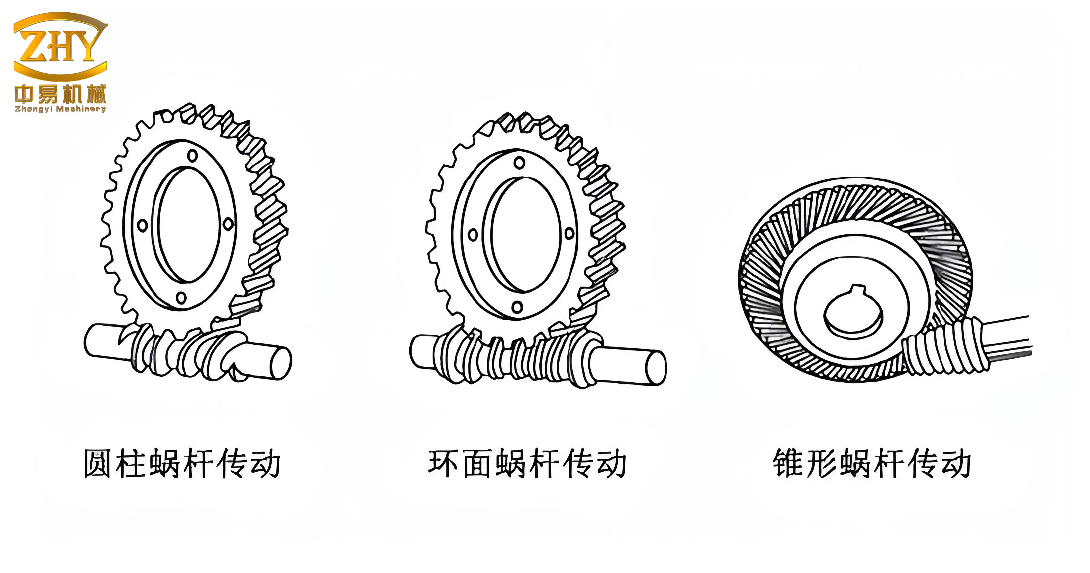
The core philosophy of my approach is generative: rather than attempting to directly sketch the complex helicoidal surface, I replicate the physical creation of the screw gear components. For the worm, this means simulating turning on a lathe. For the worm wheel, it involves simulating the gear hobbing process. Each of these manufacturing operations can be described by a definitive toolpath trajectory. By mathematically defining these paths and the cross-sectional shape of the virtual cutting tool, I can use Pro/E’s advanced sweeping and blending features to “machine” the part from a solid blank, thereby guaranteeing geometric accuracy.
Mathematical Foundation and Worm Modeling
The defining characteristic of an Archimedes worm is that its axial profile is a straight line. This aligns perfectly with its common manufacturing method: using a straight-edged lathe tool with an included angle equal to twice the worm’s axial pressure angle (\( \alpha \)). My modeling process begins by deriving the trajectory of a reference point on this cutting tool.
Consider the setup where the worm blank rotates with an angular velocity \( \omega \) about its Z-axis, while the tool translates parallel to this axis with a linear velocity \( v \). For a point \( K \) on the tool, initially at coordinates \( (r, 0, 0) \), its position after time \( t \) describes a spatial helix. The parametric equations governing this fundamental motion for the screw gear worm generation are:
$$ x = r \cdot \cos(\omega t) $$
$$ y = r \cdot \sin(\omega t) $$
$$ z = v \cdot t $$
Here, \( r \) is the radial distance of point \( K \) from the axis. The lead of the helix, which corresponds to the worm’s lead \( P_z \), is \( 2\pi v / \omega = \pi m z_1 \), where \( m \) is the module and \( z_1 \) is the number of worm starts (threads). In Pro/E, I implement this trajectory using the From Equation command under Insert a Datum Curve. I define a coordinate system and input these parametric equations directly, which creates the precise helical path that will guide the virtual cutting operation.
The next critical step is defining the cutter geometry. The cross-section of the lathe tool is determined directly from the worm’s axial tooth dimensions. Referring to the axial plane, the tool shape is a simple isosceles trapezoid (or triangle, depending on the root form) defined by the axial module \( m \), the axial pressure angle \( \alpha \), the addendum \( h_{a1} \), the dedendum \( h_{f1} \), and the axial tooth space width \( s_n \). I sketch this 2D profile in a Pro/E sketch, ensuring it is a closed loop. The key parameters are summarized in the table below:
| Parameter | Symbol | Relation/Formula |
|---|---|---|
| Axial Module | \( m \) | Design Specification |
| Number of Starts | \( z_1 \) | Design Specification |
| Axial Pressure Angle | \( \alpha \) | Design Specification (e.g., 20°) |
| Worm Addendum | \( h_{a1} \) | Typically \( 1.0m \) |
| Worm Dedendum | \( h_{f1} \) | Typically \( 1.2m \) or \( 1.25m \) |
| Axial Tooth Space Width | \( s_n \) | \( \pi m / 2 \) |
| Lead | \( P_z \) | \( \pi m z_1 \) |
| Helix Angle (at pitch cylinder) | \( \gamma \) | \( \arctan(P_z / (2\pi r_1)) = \arctan(m z_1 / d_1) \) |
With the helical path (trajectory) and the cutter section (profile) defined, I perform a Swept Blend Cut on a cylindrical worm blank. The blank’s diameter is the worm’s tip diameter \( d_{a1} \), and its length is the worm’s face width \( B_1 \). The software guides the 2D tool section along the 3D helical path, subtracting material and leaving behind the precise Archimedes spiral groove. For a multi-start screw gear worm, I create the first groove and then use a Pattern feature, rotating it around the axis \( z_1 – 1 \) times with an incremental angle of \( 360/z_1 \) degrees. The resulting model has mathematically accurate axial straight-line profiles and correct lead, fulfilling all functional requirements of the screw gear drive element.
Worm Wheel Modeling via Simulated Hobbing
Modeling the mating worm wheel is more intricate because its tooth profile is not simply an inversion of the worm’s thread. The standard manufacturing process uses a hobber, where the hob is essentially a worm with cutting edges. Therefore, modeling the worm wheel involves simulating the conjugate motion between the worm (hob) and the wheel blank. My approach is to derive the relative motion path of a point on the hob’s cutting edge as seen from the rotating worm wheel blank.
I establish two coordinate systems as shown below. System \( C_1 (O_1 – x_1, y_1, z_1) \) is fixed to the worm (hob), with \( z_1 \) along its axis. System \( C_2 (O_2 – x_2, y_2, z_2) \) is fixed to the worm wheel, with \( z_2 \) along its axis. The centers are separated by the standard center distance \( a \). The worm rotates with angular speed \( \omega_1 \), driving the wheel with angular speed \( \omega_2 \), where \( \omega_2 / \omega_1 = z_1 / z_2 \).
A cutting point \( K \) on the hob follows the same helical motion in \( C_1 \) as before. To find its path in the wheel’s coordinate system \( C_2 \), I apply a series of coordinate transformations: first a rotation of \( \omega_1 t \) in \( C_1 \), then a translation of \( -a \) along \( x_1 \), and finally a rotation of \( -\omega_2 t \) about the \( z_2 \) axis to account for the wheel’s rotation. The resulting composite motion trajectory equation for the hob point relative to the worm wheel blank is:
$$ x_2 = r_1 \cos(\omega_1 t) \cos(\omega_2 t) + a \cos(\omega_2 t) $$
$$ y_2 = r_1 \cos(\omega_1 t) \sin(\omega_2 t) + a \sin(\omega_2 t) $$
$$ z_2 = -r_1 \sin(\omega_1 t) $$
For modeling, \( v \) is substituted using the lead relation \( v = P_z \omega_1 / (2\pi) \). This complex 3D curve, which defines the path of the hob’s cutting edge through the wheel blank, is created in Pro/E using the From Equation method. This path is the master trajectory for the sweep cut that will generate the wheel tooth space.
The cross-sectional shape of the virtual hob, however, is not the same as the worm’s axial profile. In the mid-plane of the worm wheel (the plane containing the wheel axis and perpendicular to the worm axis), the meshing condition approximates that of an involute rack and pinion. Consequently, the tooth profile of the worm wheel in its own mid-plane face is an involute curve. Therefore, my virtual cutting tool for the wheel is defined by the 2D involute tooth space profile in its mid-plane.
I generate a single-side involute profile using the Pro/E equation curve function with the standard parametric involute equations in Cartesian form:
$$ x = r_b (\cos(\theta_k) + \theta_k \sin(\theta_k)) $$
$$ y = r_b (\sin(\theta_k) – \theta_k \cos(\theta_k)) $$
$$ z = 0 $$
Here, \( r_b \) is the base circle radius of the worm wheel (\( r_b = r_2 \cos\alpha \), where \( r_2 \) is the pitch radius and \( \alpha \) is the normal pressure angle), and \( \theta_k \) is the involute roll angle. To create the full tooth space (groove) profile, I need the angular thickness of the tooth space on the base circle. The tooth thickness \( s_k \) at any arbitrary radius \( r_k \) is calculated from the known thickness at the pitch circle (\( s_2 = \pi m / 2 \)):
$$ s_k = r_k \left( \frac{s_2}{r_2} + 2 (\text{inv}(\alpha) – \text{inv}(\alpha_k)) \right) $$
where \( \alpha_k = \arccos(r_b / r_k) \) and \( \text{inv}(x) = \tan(x) – x \) is the involute function. The angular extent of the tooth space on the base circle \( \theta_{space} \) is \( s_b / r_b \). I use this angle to position a mirror plane, allowing me to mirror the single involute curve and create a symmetric, closed tooth space profile. This closed profile becomes the cross-section of my virtual hob for the wheel.
The final modeling step for the worm wheel is to perform a Swept Blend Cut on a cylindrical wheel blank (diameter = tip diameter \( d_{a2} \), width = face width \( B_2 \)). I use the complex 3D hobbing trajectory derived earlier as the sweep path and the 2D involute tooth space as the cross-section. Pro/E then simulates the material removal along this conjugate path. The resulting feature is a single, perfectly formed tooth space. I then create a circular Pattern of this cut feature around the wheel axis with a count equal to the number of teeth \( z_2 \). This completes the precise generation of the worm wheel, ready for assembly with its mating worm to form a fully functional virtual screw gear drive. The table below summarizes the key equations and parameters used in the worm wheel synthesis.
| Element | Mathematical Definition / Key Parameter |
|---|---|
| Hob Path in Wheel Coords | $$ \begin{aligned} x_2 &= r_1 \cos(\omega_1 t) \cos(\omega_2 t) + a \cos(\omega_2 t) \\ y_2 &= r_1 \cos(\omega_1 t) \sin(\omega_2 t) + a \sin(\omega_2 t) \\ z_2 &= -r_1 \sin(\omega_1 t) \end{aligned} $$ |
| Wheel Involute Profile | $$ \begin{aligned} x &= r_b (\cos\theta + \theta \sin\theta) \\ y &= r_b (\sin\theta – \theta \cos\theta) \\ r_b &= r_2 \cos\alpha_n \end{aligned} $$ |
| Tooth Thickness at Radius \( r_k \) | $$ s_k = r_k \left( \frac{s_2}{r_2} + 2 (\text{inv}(\alpha) – \text{inv}(\alpha_k)) \right) $$ |
| Center Distance | \( a = (d_1 + d_2)/2 = m(q + z_2)/2 \) where \( q \) is the diameter quotient. |
Application, Assembly, and Verification
Once both components of the screw gear pair are modeled, their utility in the digital engineering workflow becomes evident. I first create the full shaft model for the worm, adding bearing journals, keyways, and other manufacturing features to the “threaded” section generated earlier. Similarly, for the worm wheel, I design the web, hub, bolt holes, and other structural details around the geared rim.
The critical test is the virtual assembly. I constrain the worm and wheel models using Pro/E’s assembly module: aligning their axes at the specified center distance \( a \), and creating a gear pair connection with a defined gear ratio \( z_2:z_1 \). Successful assembly without interference in the initial position is a good first indicator. I then run a global interference check and a dynamic clearance analysis through a range of rotational motion. The absence of collision and the maintenance of proper backlash confirm that the models are geometrically conjugate and accurately represent a functional Archimedes screw gear set.
These precise models serve as the foundation for advanced engineering analyses. They can be directly used for Finite Element Analysis (FEA) to study contact stresses, bending stresses, and thermal deformation under load. The accurate geometry ensures that load application and boundary conditions in the simulation reflect real-world behavior. Furthermore, the assembly can be used in multi-body dynamics software for motion simulation, efficiency calculation, and vibration analysis, providing invaluable insights early in the design process.
The methodology I’ve described is not limited to the Archimedes type. The principle of simulating the manufacturing trajectory is universally applicable. For example, modeling an involute helical gear (another common screw gear variant) would involve defining a helical path with a lead equal to the gear’s lead and using an involute cutter profile. The same Pro/E tools—From Equation curves and Swept Blend—are employed. This makes the approach a powerful general framework for precise gear modeling.
Conclusion
My exploration into precise 3D modeling of the Archimedes screw gear drive within Pro/E demonstrates that a deep understanding of the component’s generative geometry is more effective than relying solely on standard CAD features or embarking on lengthy API development. By deriving the mathematical equations that govern the manufacturing toolpaths—a simple helix for the worm and a complex conjugated spatial curve for the wheel—and leveraging Pro/E’s equation-driven curve and advanced sweeping capabilities, I can construct digital models that are exact geometric counterparts to physically manufactured parts.
This first-principles approach ensures the model’s fidelity, which is critical for downstream applications like interference checking, FEA, and dynamic simulation. The technique is robust, repeatable, and adaptable to other types of gears, making it an essential strategy in the toolkit of any mechanical designer or analyst working with precision power transmission elements like the screw gear. The ability to move seamlessly from design parameters to a verifiable, analyzable 3D assembly significantly accelerates the development cycle and enhances the reliability of mechanical systems employing worm and worm wheel drives.