
The pursuit of superior meshing performance in gear drives is a cornerstone of advanced mechanical design, particularly for applications demanding high power density, smooth operation, and minimal noise and vibration. Among various gear types, the hyperboloid gear, or hypoid gear, holds a distinguished position, especially in automotive final drives. Its defining characteristic is the offset between the axes of the pinion and the gear, which allows for a lower center of gravity in vehicles, enhancing stability, or provides greater ground clearance in off-road applications. This geometric complexity, however, translates into a significantly more challenging design and manufacturing process compared to parallel-axis or intersecting-axis gears. The quality of meshing—encompassing the contact pattern, transmission error, and sensitivity to misalignments—is not inherent in the blank design but is fundamentally imparted during the cutting process through the precise configuration of machine-tool settings. Therefore, the development of a systematic methodology for determining optimal cutting parameters is paramount for realizing the full potential of hyperboloid gear drives.
This article delves into the cutting design for a specific, high-potential manufacturing method known as the Hypoid Generated Tilt (HGT) process. In the HGT method, the gear (typically the larger member) is generated using a dual-sided cutter head, which produces a fully conjugate, curvature-rich tooth surface. While slightly less efficient than non-generated (Formate) methods, this generation process offers superior control over the local surface geometry. The pinion is then cut using a single-sided cutter head with a titling mechanism (tilt and swivel). This combination leverages the benefits of generation for quality and tilt for simplified tooling and adjustment flexibility. The core challenge is to calculate the precise set of machine-tool settings—horizontal and vertical cradle offsets, radial and angular settings, machine root angles, ratio coefficients, and tilt angles—that will yield a hyperboloid gear pair with predetermined, high-quality meshing properties. The methodology adopted here is rooted in the powerful Local Synthesis technique, which allows for the pre-control of meshing conditions at a designated reference point and its immediate vicinity on the tooth flank.
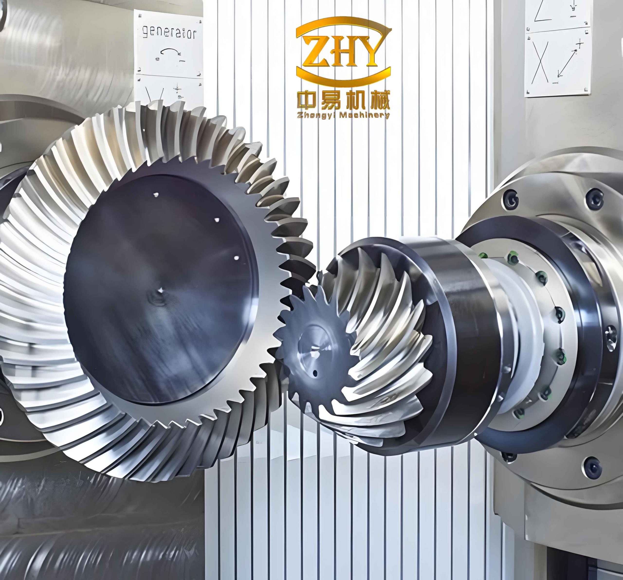
The principle of Local Synthesis is a systematic procedure for designing the pinion tooth surface to mesh correctly with a given gear tooth surface under specified contact conditions. It operates on differential geometry and gear meshing theory. The process begins with a fully defined gear tooth surface, produced according to standard cutting parameters. A reference point \( M \) is chosen on this gear surface. The first-order contact parameter is the location of \( M \), which essentially determines the center of the contact pattern. At point \( M \), the principal curvatures \( k_f^{(2)}, k_h^{(2)} \) and principal directions \( \mathbf{e}_f^{(2)}, \mathbf{e}_h^{(2)} \) of the gear tooth surface are calculated. Then, three second-order contact parameters are prescribed:
1. The derivative of the transmission function at \( M \), denoted \( m_{21}’ \). This parameter controls the slope and symmetry of the transmission error curve.
2. The angle \( \eta_2 \) between the contact path (on the gear) and the root line. This angle influences the length of the contact pattern and the overlap ratio.
3. The semi-major axis length \( a \) of the contact ellipse at \( M \). This parameter governs the width of the contact pattern and the contact stress level.
Using the fundamental relations of point contact between two surfaces, the required principal curvatures \( k_I^{(1)}, k_{II}^{(1)} \) and principal directions \( \mathbf{e}_I^{(1)}, \mathbf{e}_{II}^{(1)} \) for the pinion tooth surface at the conjugate point \( M \) are computed. The final and most crucial step is to back-calculate the pinion machine-tool settings that will produce a pinion tooth surface possessing exactly these local geometric properties at \( M \). This method ensures that the desired meshing performance is “built into” the pinion surface from the start.
The first phase in applying Local Synthesis to HGT hyperboloid gears is the complete definition of the gear cutting process and its surface. The gear is generated on a hypoid generator using a dual-sided cutter head. The coordinate systems involved are shown in the conceptual figure below. The machine coordinate system \( O_{c2}-X_{c2}Y_{c2}Z_{c2} \) is fixed to the cradle. The cutter head, with center \( O_g \), rotates about its own axis while the cradle rotates with angle \( \phi_2 \), generating the gear tooth surface via the rolling motion between the imaginary generating gear (represented by the cradle) and the gear blank. Standard gear blank geometry parameters are used as input.
The primary machine settings for the gear are determined from basic gear geometry. Given the mean cone distance \( A_m \), spiral angle \( \beta_2 \), and cutter radius \( R_{G2} \), the basic cradle offsets are:
$$ H_2 = (A_m + \Delta x) \cos \theta_{r2} – R_{G2} \sin \beta_2 $$
$$ V_2 = R_{G2} \cos \beta_2 $$
where \( \theta_{r2} \) is the root angle and \( \Delta x \) is an offset from the mean point along the face width, initially zero. The radial and angular settings are then:
$$ S_{r2} = \sqrt{H_2^2 + V_2^2}, \quad q_2 = \sin^{-1}(V_2 / S_{r2}) $$
Other essential settings like the sliding base (or axial) setting \( X_{G2} \), the machine center to back (or blank) setting \( X_{B2} \), and the ratio \( C_{r2} \) are derived from the gear’s pitch cone and root cone geometry. Once these parameters are set, the gear tooth surface \( \Sigma_2 \) is mathematically defined by its generating motion.
The next critical step is selecting the reference point \( M \). It is defined by its longitudinal (\( X_L \)) and profile (\( H_L \)) coordinates relative to the mean point \( M_0 \):
$$ X_L = X_{M_0} + \Delta x, \quad H_L = Y_{M_0} + \Delta y $$
By varying \( \Delta x \) and \( \Delta y \), the designer can strategically position the core of the contact pattern. For example, a positive \( \Delta x \) shifts the reference point towards the toe, while a positive \( \Delta y \) shifts it towards the topland. The corresponding cradle rotation angle \( \phi_2^{(M)} \) and cutter point coordinates for point \( M \) are calculated based on its location.
The local geometry of the gear surface at \( M \) must be determined. The cutter blade surface is a cone. For a blade with pressure angle \( \alpha_2 \), its position vector \( \mathbf{r}_g \) and unit normal \( \mathbf{n}_g \) in the cutter coordinate system are parameterized by the blade setting distance \( S_g \) and rotation angle \( \theta_g \):
$$ \mathbf{r}_g = \begin{bmatrix} (r_{c2} – S_g \sin \alpha_2) \cos \theta_g \\ (r_{c2} – S_g \sin \alpha_2) \sin \theta_g \\ -S_g \cos \alpha_2 \\ 1 \end{bmatrix}, \quad \mathbf{n}_g = \begin{bmatrix} -\cos \alpha_2 \cos \theta_g \\ -\cos \alpha_2 \sin \theta_g \\ \sin \alpha_2 \end{bmatrix} $$
Its principal directions and curvatures are:
$$ \mathbf{e}_s^{(g)} = \begin{bmatrix} -\sin \theta_g \\ \cos \theta_g \\ 0 \end{bmatrix}, \quad \mathbf{e}_q^{(g)} = \begin{bmatrix} -\sin \alpha_2 \cos \theta_g \\ -\sin \alpha_2 \sin \theta_g \\ -\cos \alpha_2 \end{bmatrix} $$
$$ k_s^{(g)} = \frac{\cos \alpha_2}{r_{c2} – S_g \sin \alpha_2}, \quad k_q^{(g)} = 0 $$
These entities are transformed through the sequence of coordinate systems: from cutter to machine (\( \mathbf{M}_{c2g} \)), then from machine to the gear (\( \mathbf{M}_{2c2} \)), and finally to the fixed meshing coordinate system \( O_h – X_hY_hZ_h \) (\( \mathbf{M}_{h2} \)). The transformation matrix to the machine coordinate system is:
$$ \mathbf{M}_{c2g} = \begin{bmatrix} \cos \gamma_2 \cos \phi_g & \cos \gamma_2 \sin \phi_g & \sin \gamma_2 & \cos \gamma_2 (H_2 \cos \phi_g + V_2 \sin \phi_g) – X_{B2} \sin \gamma_2 \\ -\sin \phi_g & \cos \phi_g & 0 & -H_2 \sin \phi_g + V_2 \cos \phi_g \\ -\sin \gamma_2 \cos \phi_g & -\sin \gamma_2 \sin \phi_g & \cos \gamma_2 & -\sin \gamma_2 (H_2 \cos \phi_g + V_2 \sin \phi_g) – X_{B2} \cos \gamma_2 \\ 0 & 0 & 0 & 1 \end{bmatrix} $$
After these transformations, we obtain the gear surface’s position vector \( \mathbf{r}_h^{(2)} \), unit normal \( \mathbf{n}_h^{(2)} \), and most importantly, its principal curvatures \( k_I^{(2)}, k_{II}^{(2)} \) and principal directions \( \mathbf{e}_I^{(2)}, \mathbf{e}_{II}^{(2)} \) expressed in the meshing coordinate system. This completes the characterization of the given member of the hyperboloid gear pair.
The core of the Local Synthesis algorithm is now executed. The three second-order parameters \( (m_{21}’, \eta_2, a) \) are input as design goals. Using the classical relations for the contact of two surfaces, the required principal curvatures and directions for the pinion surface at the conjugate point are solved. The governing equations stem from the condition that the relative normal curvature in any direction \( \boldsymbol{\nu} \) on the tangent plane is related to the principal curvatures of both surfaces and the angle between their principal directions. The system ensures that the contact ellipse at \( M \) has the prescribed orientation (\( \eta_2 \)) and size (\( a \)), and that the transmission error has the prescribed slope (\( m_{21}’ \)). The results of this calculation are the pinion’s principal curvatures \( k_I^{(1)}, k_{II}^{(1)} \), principal directions \( \mathbf{e}_I^{(1)}, \mathbf{e}_{II}^{(1)} \), and the angle \( \sigma^{(12)} \) between the first principal directions of the gear and pinion.
With the target pinion surface geometry at point \( M \) known, the next step is to find the cutter geometry and machine settings that will produce it. The pinion is cut using a single-sided cutter head with a titling mechanism. The pinion cutter surface is also a cone. The condition of line contact between the imaginary generating surface (the cutter) and the desired pinion surface during the generation process is invoked. This allows the calculation of the required principal curvatures \( k_I^{(p)}, k_{II}^{(p)} \) and directions \( \mathbf{e}_I^{(p)}, \mathbf{e}_{II}^{(p)} \) for the cutter surface, as well as the angle \( \sigma^{(p1)} \) between the cutter’s and pinion’s first principal directions.
From the geometry of the conical cutter blade with pressure angle \( \alpha_1 \), these curvatures and directions directly define the cutter axis orientation and the location of the cutter center relative to the meshing point. The unit vector of the cutter axis \( \mathbf{C}_h^{(p)} \) and the position vector of the cutter center \( \mathbf{R}_h^{(p)} \) are found from:
$$ \mathbf{C}_h^{(p)} = -\mathbf{e}_I^{(F)} \cos \alpha_1 – \mathbf{n}_h^{(1)} \sin \alpha_1 $$
$$ \mathbf{R}_h^{(p)} = \mathbf{r}_h^{(1)} – \mathbf{e}_I^{(F)} (S_p + r_{c1}^{(1)} \sin \alpha_1) + \mathbf{n}_h^{(1)} r_{c1}^{(1)} \cos \alpha_1 $$
Here, \( \mathbf{r}_h^{(1)} = \mathbf{r}_h^{(2)} \) and \( \mathbf{n}_h^{(1)} = -\mathbf{n}_h^{(2)} \) at the contact point \( M \), \( S_p \) is the blade point radius parameter, and \( r_{c1}^{(1)} \) is the cutter point radius.
These vectors, \( \mathbf{C}_h^{(p)} \) and \( \mathbf{R}_h^{(p)} \), are then transformed into the pinion machine coordinate system. The sequence involves transformation to an intermediate system aligned with the initial machine setup \( (\mathbf{M}_{qh}) \), and then to the final machine system \( (\mathbf{M}_{c1q}) \). The tilt angle \( i \) and swivel angle \( j \) are extracted directly from the components of the cutter axis vector \( \mathbf{C}_q^{(p)} = [C_{qx}^{(p)}, C_{qy}^{(p)}, C_{qz}^{(p)}]^T \):
$$ i = \sin^{-1} \left( \sqrt{ (C_{qx}^{(p)})^2 + (C_{qy}^{(p)})^2 } \right) $$
$$ j = \tan^{-1} \left( -C_{qy}^{(p)} / C_{qx}^{(p)} \right) $$
The machine settings for horizontal offset \( H_1 \), vertical offset \( V_1 \), and sliding base \( X_{b1} \) are the components of the cutter center location vector \( \mathbf{R}_{c1}^{(p)} \):
$$ H_1 = R_{c1x}^{(p)}, \quad V_1 = R_{c1y}^{(p)}, \quad X_{b1} = R_{c1z}^{(p)} $$
The radial and angular settings follow as:
$$ S_{r1} = \sqrt{H_1^2 + V_1^2}, \quad q_1 = \sin^{-1}(V_1 / S_{r1}) $$
Finally, the ratio \( C_{r1} \), axial setting \( X_{g1} \), and vertical offset \( E_{m1} \) are determined by satisfying the equation of meshing between the pinion cutter and the pinion blank during the generation process, \( \mathbf{v}^{(p1)} \cdot \mathbf{n}_{c1}^{(1)} = 0 \), where \( \mathbf{v}^{(p1)} \) is the relative velocity. Solving this equation, along with the known geometry, yields the final machine-tool settings for the pinion. This completes the synthesis loop for the HGT hyperboloid gear pair.
To validate the methodology, a design example is performed. The basic blank data for a typical automotive hypoid gear set is used as input.
| Blank Parameter | Gear | Pinion |
|---|---|---|
| Number of Teeth | 39 | 7 |
| Face Width (mm) | 63 | 68 |
| Mean Cone Distance (mm) | 190.938 | 180.343 |
| Shaft Angle (°) | 90 | |
| Offset (mm) | 35 | |
The Local Synthesis control parameters are chosen to achieve favorable performance: a contact path angle \( \eta_2 = 35^\circ \) for good overlap, a transmission error slope \( m_{21}’ = -0.0004 \) for a symmetric, low-magnitude error curve, and a contact ellipse semi-major axis set to 30% of the face width. The reference point is initially placed near the center of the flank (\( \Delta x = 0, \Delta y = 0 \)). Applying the described procedure yields the complete set of machine-tool settings.
| Machine-Tool Setting | Gear (Generated) | Pinion (HGT Cut) |
|---|---|---|
| Cutter Blade Angle (°) | 22.500 | 14.000 |
| Cutter Radius (mm) | 152.400 | 165.257 |
| Horizontal Offset (mm) | 104.506 | 45.831 |
| Vertical Offset (mm) | 0 | -4.921 |
| Tilt Angle i (°) | – | 5.314 |
| Swivel Angle j (°) | – | -109.948 |
| Ratio | 0.978 | 0.234 |
Tooth Contact Analysis (TCA) is performed on the virtual gear pair defined by these settings. TCA simulates the meshing of the theoretical tooth surfaces under load-free conditions. The results show a well-centered contact pattern with a straight path of contact closely aligned to the desired \( 35^\circ \) angle, indicating low sensitivity to misalignment. The transmission error curve is parabolic with a small amplitude and is symmetric, confirming smooth and quiet operation. No edge contact is predicted.
The power of the active design approach is demonstrated by changing a control parameter. If the reference point is shifted towards the toe and topland (\( \Delta x = 3 \text{ mm}, \Delta y = 2 \text{ mm} \)), the Local Synthesis procedure is repeated. The gear settings remain unchanged, but a new set of pinion machine settings is calculated automatically. The resulting TCA shows the contact pattern has correspondingly shifted, as intended, while still maintaining a favorable straight path and a low, symmetric transmission error. This confirms that the meshing performance of the hyperboloid gear drive can be precisely targeted and controlled through the strategic selection of Local Synthesis parameters.
In conclusion, the integration of the Hypoid Generated Tilt (HGT) manufacturing method with the Local Synthesis design philosophy provides a robust and systematic framework for producing high-performance hyperboloid gear drives. The HGT method itself offers an excellent balance: the generated gear member ensures superior, controllable flank geometry, while the tilted single-sided cutting of the pinion simplifies tooling logistics. The Local Synthesis algorithm is the key that unlocks this potential. By allowing the engineer to pre-specify critical second-order meshing characteristics—such as contact path direction, transmission error curve shape, and contact ellipse size—at a chosen reference point, it moves gear design from a trial-and-error adjustment process to a precise, predictive science. The calculated machine-tool settings are optimal in the sense that they are derived directly from the desired functional performance. This methodology ensures that the final hyperboloid gear pair will exhibit a long, straight contact pattern for high durability and low misalignment sensitivity, along with a low-amplitude, parabolic transmission error function for smooth and quiet operation. It represents a significant tool for advancing the design and manufacture of these complex yet indispensable power transmission components.