
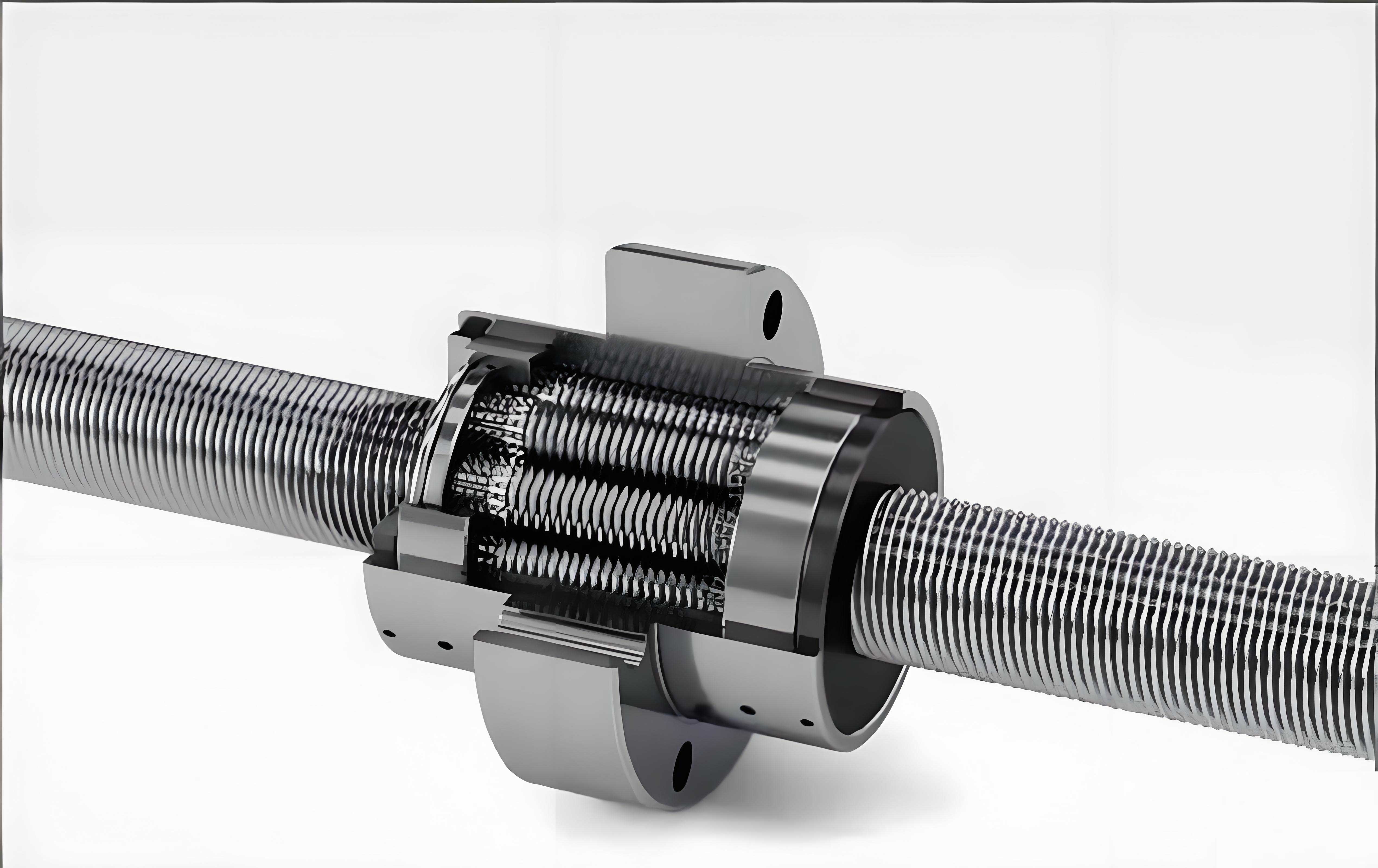
In my research into high-performance mechanical transmissions, I have focused extensively on the planetary roller screw assembly. This mechanism is a superior actuator for converting rotary motion into linear motion, offering exceptional load capacity, stiffness, and longevity compared to traditional ball screws. Its structure is an elegant synthesis of planetary gear kinematics and screw thread mechanics. However, achieving optimal performance in a planetary roller screw assembly is critically dependent on controlling the meshing contact state between its three primary components: the central screw, the planetary rollers, and the surrounding nut. Misalignment or improper geometry leads to interference, which increases preload, accelerates wear, and reduces efficiency, or excessive backlash, which compromises positioning accuracy. Therefore, a precise method for calculating and controlling the meshing geometry is paramount for the successful design and planetary roller screw assembly process.
The core challenge stems from the spatial nature of the contact. The threads on the screw, rollers, and nut are complex spatial helical surfaces. The theoretical meshing point, where these surfaces should ideally make contact, often shifts due to manufacturing tolerances and the compound planetary motion of the rollers. This shift can cause severe interference during the planetary roller screw assembly. While prior studies have approached this by discretizing the contact zone into planar sections or analyzing contact points using Frenet frames, a method that directly and precisely calculates the axial clearance or interference between the discretized spatial surfaces offers a more intuitive and computationally manageable solution for practical engineering applications.
Fundamental Components and Motion Principles
A standard planetary roller screw assembly consists of a central screw with multiple-start threads, several planetary rollers with single-start threads distributed around it, and a nut with internal threads engaging the rollers. The rollers are retained in a cage that maintains their angular positions relative to each other, allowing them to orbit the screw axis while also rotating about their own axes. The kinematic relationship dictates that for one revolution of the screw relative to the nut, the rollers undergo a compound motion involving both planetary revolution and self-rotation. The fundamental geometric parameters defining a planetary roller screw assembly are listed in Table 1.
| Geometric Parameter | Symbol (Screw/Roller/Nut) | Description |
|---|---|---|
| Pitch | $$P_0$$ | Basic distance between corresponding points on adjacent threads. |
| Number of Thread Starts | $$n_s$$ / 1 / $$n_n$$ | Number of independent helical threads. Rollers are typically single-start. |
| Lead | $$P_s = n_s P_0$$ / $$P_r = P_0$$ / $$P_n = n_n P_0$$ | Axial distance traveled per revolution of the component. |
| Thread Flank Angle | $$\beta$$ | Half-angle of the thread profile (commonly 45°). |
| Pitch Diameter (Nominal) | $$d_s$$ / $$d_r$$ / $$d_n$$ | Theoretical diameter at which thread thickness equals space width. |
| Profile Radius (Roller) | $$R_r$$ | Radius of the circular arc forming the roller thread profile. |
| Center Distance | $$a = \frac{d_s + d_r}{2}$$ | Nominal distance between screw and roller axes. |
The motion transmission relies on the precise conjugate meshing of these helical surfaces. Any deviation from the ideal geometry disrupts this conjugate action, leading to the interference problem central to the planetary roller screw assembly challenge.
Mathematical Modeling of Helical Surfaces
To analyze the contact, I first establish a mathematical model for the thread surfaces. A spatial coordinate system is defined, as shown in Figure 1 (conceptually). It includes a fixed global frame $$(Oxyz)$$, a frame attached to the roller $$(O_Rx_Ry_Rz_R)$$, and profile frames for the screw, roller, and nut. The key to describing the planetary roller screw assembly geometry is representing the helical surfaces parametrically.
Consider the left-side flank of a roller thread. A point $$M$$ on its generating profile in the roller’s profile frame has coordinates:
$$
\begin{align*}
x_{rM}(u_r) &= R_r \sin u_r – R_r \sin \beta + r_r \\
y_{rM}(u_r) &= 0 \\
z_{rM}(u_r) &= -\frac{P_0}{4} + R_r \cos \beta – R_r \cos u_r
\end{align*}
$$
where $$u_r$$ is an angular parameter along the circular profile, and $$r_r = d_r/2$$ is the roller pitch radius. When this profile undergoes a screw motion about the roller axis, it generates the left helical surface of the roller, given by:
$$
\vec{S}_r(u_r, \theta_r) =
\begin{bmatrix}
(R_r \sin u_r – R_r \sin \beta + r_r) \cos \theta_r \\
(R_r \sin u_r – R_r \sin \beta + r_r) \sin \theta_r \\
-\frac{P_0}{4} + R_r \cos \beta – R_r \cos u_r + \frac{P_r}{2\pi}\theta_r
\end{bmatrix}, \quad \theta_r \in [0, 2\pi]
$$
Here, $$\theta_r$$ is the rotation angle parameterizing the helix.
Similarly, the right-side flank of the screw thread can be modeled as a straight-line profile undergoing a screw motion. Its surface equation is:
$$
\vec{S}_s(u_s, \theta_s) =
\begin{bmatrix}
(u_s \cos \beta + r_s) \cos \theta_s \\
(u_s \cos \beta + r_s) \sin \theta_s \\
\frac{P_0}{4} + u_s \sin \beta + \frac{P_s}{2\pi}\theta_s
\end{bmatrix}
$$
where $$u_s$$ is a linear parameter along the straight flank, and $$r_s = d_s/2$$. The nut’s right-side flank surface $$\vec{S}_n(u_n, \theta_n)$$ has an identical form, substituting $$r_n$$ and $$P_n$$.
The coordinate transformation between the roller frame and the fixed frame is essential for analyzing the planetary roller screw assembly meshing. It is given by the homogeneous transformation matrix:
$$
\begin{bmatrix} x \\ y \\ z \\ 1 \end{bmatrix} =
\begin{bmatrix}
1 & 0 & 0 & a \\
0 & 1 & 0 & 0 \\
0 & 0 & 1 & 0 \\
0 & 0 & 0 & 1
\end{bmatrix}
\begin{bmatrix} x_R \\ y_R \\ z_R \\ 1 \end{bmatrix}
$$
where $$a$$ is the center distance between the screw and roller axes. This transformation allows us to express the roller’s helical surface in the same global coordinate system as the screw and nut surfaces, enabling direct comparison and interference calculation critical for the planetary roller screw assembly.
Discretization-Based Meshing State Calculation Algorithm
Direct analytical solution for the contact between two complex 3D helical surfaces in a planetary roller screw assembly is exceedingly difficult. My approach simplifies this by discretizing the potential contact zone on the helical surfaces into a dense cloud of points and then calculating the axial distance between corresponding points. The procedure for the screw-roller pair is detailed below, and the nut-roller pair follows the same logic.
Step 1: Discretization of the Contact Zone. The contact does not occur over the entire thread surface. I identify the probable contact region in the XY-plane (transverse cross-section), as illustrated in Figure 3. This region is discretized into a finite set of grid points $$P_{RSi}(x_{RSi}, y_{RSi})$$. This focused discretization significantly reduces computational load while capturing all relevant geometry for the planetary roller screw assembly analysis.
Step 2: Calculation of Axial Coordinates. For each discrete point $$P_{RSi}$$, I find the corresponding axial (Z) coordinate on both the screw and roller helical surfaces. This involves solving the surface equations for $$z$$ given the known $$x$$ and $$y$$ coordinates. For the roller surface transformed into the global frame, we solve:
$$
\begin{cases}
x = (R_r \sin u_r – R_r \sin \beta + r_r) \cos \theta_r + a = x_{RSi} \\
y = (R_r \sin u_r – R_r \sin \beta + r_r) \sin \theta_r = y_{RSi}
\end{cases}
$$
for the parameters $$u_r$$ and $$\theta_r$$, and then substitute them into the $$z$$-component equation to get $$z_{Ri}$$. For the screw surface, we solve:
$$
\begin{cases}
x = (u_s \cos \beta + r_s) \cos \theta_s = x_{RSi} \\
y = (u_s \cos \beta + r_s) \sin \theta_s = y_{RSi}
\end{cases}
$$
for $$u_s$$ and $$\theta_s$$ to obtain $$z_{Si}$$. This yields two points in space: $$P_{Ri}(x_{RSi}, y_{RSi}, z_{Ri})$$ on the roller and $$P_{Si}(x_{RSi}, y_{RSi}, z_{Si})$$ on the screw, which share the same projection in the XY-plane.
Step 3: Determination of Interference/Gap and Contact Point. The axial clearance or interference at this projected location is simply the difference: $$\Delta z_i = z_{Si} – z_{Ri}$$.
- If $$\Delta z_i > 0$$, there is a clearance (gap) of that magnitude.
- If $$\Delta z_i < 0$$, there is an interference (overlap) of that magnitude.
The actual meshing contact point in this discrete model is the point $$P_{RSi}$$ where the absolute value of $$\Delta z_i$$ is minimized. By iterating this calculation over all discrete points in the contact zone, I can map the entire meshing state and accurately quantify the maximum interference or minimum clearance present in the planetary roller screw assembly.
Step 4: Iterative Parameter Adjustment. The core utility of this algorithm for the planetary roller screw assembly lies in its iterative application. By varying key design parameters—most effectively the pitch diameters $$d_s$$ and $$d_n$$—and re-running the calculation, I can determine the exact parameter values that yield a desired meshing state, such as zero clearance (perfect theoretical contact) or a specific preload interference. This process replaces trial-and-error in physical assembly with precise digital simulation.
Algorithm Verification via Virtual Assembly
To validate the accuracy of my discretization algorithm, I conducted a comparative study using the geometric parameters from a typical design, as shown in Table 2.
| Component | Pitch Diameter (mm) | Lead (mm) | Starts | Flank Angle (°) | Profile Radius (mm) |
|---|---|---|---|---|---|
| Screw | 19.5000 | 5 (Pitch=1) | 5 | 45 | – |
| Roller | 6.5000 | 1 | 1 | ||
| Nut | 32.5000 | 5 | 5 |
Using the nominal center distance $$a = (19.5+6.5)/2 = 13.0 \text{ mm}$$, my algorithm predicted significant interference between the screw and roller. To verify, I created precise 3D CAD models based on these parameters and performed a virtual planetary roller screw assembly in SolidWorks, using its interference detection tool. The results from both methods as I adjusted the screw pitch diameter are compared in Table 3. My algorithm reports the minimum axial distance (negative for interference), while SolidWorks reports an interference volume.
| Screw Pitch Diameter (mm) | Virtual Assembly Interference Volume (mm³) | Proposed Algorithm Min. Axial Distance (mm) |
|---|---|---|
| 19.50000 | 2.17 | -2.07 × 10⁻² |
| 19.49000 | 1.25 × 10⁻³ | -1.57 × 10⁻² |
| 19.48000 | 5.81 × 10⁻⁴ | -1.07 × 10⁻² |
| 19.47000 | 1.66 × 10⁻⁴ | -5.70 × 10⁻³ |
| 19.46000 | 2.71 × 10⁻⁶ | -7.31 × 10⁻⁴ |
| 19.4586 | 5.46 × 10⁻⁹ | -3.13 × 10⁻⁵ |
| 19.45854 | ~4 × 10⁻¹¹ | -1.25 × 10⁻⁶ |
| 19.45852 | 0 (No Interference) | +8.75 × 10⁻⁶ |
The correlation is excellent. Both methods converge on a near-zero interference condition when the screw pitch diameter is approximately 19.45852 mm. My algorithm demonstrates superior sensitivity, capable of resolving axial clearances on the order of 10⁻⁶ mm, far exceeding the 0.001 mm precision typically required in engineering. This validates the algorithm as a reliable and highly precise tool for analyzing the planetary roller screw assembly meshing condition.
Elimination of Interference through Pitch Diameter Adjustment
The verification study confirms the initial problem: assembling a planetary roller screw assembly with nominal theoretical pitch diameters results in substantial interference. My analysis provides a clear and effective solution: controlled adjustment of the component pitch diameters.
For the screw-roller interface, reducing the screw pitch diameter $$d_s$$ eliminates interference. Crucially, my calculations show that this adjustment does not alter the transverse (XY-plane) coordinates of the meshing point. It only changes the axial phase relationship between the screw and roller helices, bringing them into alignment without contact point shift. This is vital because it means the fundamental kinematics and load distribution of the planetary roller screw assembly remain unchanged.
Figure 5 conceptually illustrates this effect. With the nominal diameter (19.5 mm), a large area of interference (negative axial distance) exists. After optimizing the diameter to approximately 19.4585 mm, the interference zone shrinks dramatically, converging to a near-perfect point contact. The minimum axial distance is brought to virtually zero (e.g., -3.3×10⁻⁵ mm), which is functionally equivalent to perfect theoretical contact for a lubricated planetary roller screw assembly.
Conversely, the nut-roller interface with nominal parameters typically shows no interference or even a slight clearance. Therefore, the nut pitch diameter $$d_n$$ becomes the primary control parameter for introducing a desired preload. By slightly increasing $$d_n$$, a controlled interference (preload) can be generated at the nut-roller interface to eliminate overall system backlash without affecting the screw-roller meshing point location. This two-step adjustment—optimizing $$d_s$$ for zero interference at the screw-roller interface, then tuning $$d_n$$ for the desired system preload—provides a complete and rational methodology for the geometric design of a high-performance planetary roller screw assembly.
| Condition | Screw Pitch Diameter (mm) | Min. Axial Distance Screw-Roller (mm) | Meshing Point (XY Projection) | Contact Quality |
|---|---|---|---|---|
| Nominal (Theoretical) | 19.50000 | -0.0207 | (9.7648, 0.3191) | Severe Area Interference |
| Adjusted (Optimized) | ~19.4585 | ~ -3 × 10⁻⁵ | (9.7648, 0.3191) | Near-Point Contact, No Functional Interference |
Conclusion
In this work, I have developed and validated a precise, practical methodology for analyzing and controlling the meshing state in a planetary roller screw assembly. The core of the method is the discretization of the helical contact surfaces and the direct calculation of axial clearances, which bypasses the complexity of full analytical contact mechanics. This algorithm achieves a computational precision far exceeding practical manufacturing tolerances (down to 10⁻⁵ mm), providing a reliable digital tool for design.
The key findings with direct implications for the planetary roller screw assembly are:
- Interference is Inherent with Nominal Geometry: Assembling components using textbook pitch diameter formulas leads to significant interference, confirming a fundamental design challenge.
- Pitch Diameter Adjustment is the Optimal Solution: Compensating by slightly reducing the screw pitch diameter ($$d_s$$) effectively eliminates screw-roller interference without altering the kinematic contact path.
- Independent Preload Control: The nut pitch diameter ($$d_n$$) can be independently adjusted to introduce a controlled preload, allowing backlash elimination and stiffness tuning.
- Methodology Validation: The excellent agreement between the algorithm’s predictions and virtual CAD assembly results confirms its accuracy and utility as a design tool.
This approach transforms the planetary roller screw assembly process from one of trial-and-error and selective fitting into a predictable, precision engineering task. By calculating the required pitch diameter adjustments beforehand, manufacturers can machine components to the correct dimensions, ensuring a proper meshing state upon first assembly. This enhances performance, reliability, and manufacturing yield for these critical high-end mechanical actuators.