
I begin with a practical engineering problem: a compact robotic joint uses a train of straight bevel gears to transfer motion from a concentrated motor set to two output rotation axes. The performance of the joint depends strongly on the tooth geometry, contact behavior, and dynamic response of those straight bevel gears. My goal is therefore to build an accurate parametric model of the straight bevel gears, verify the assembly without interference, simulate the gear train under realistic motion and load, and then examine the contact stress of the most critical straight bevel gear pair. I treat the straight bevel gears not as decorative CAD components but as precise transmission elements whose spherical involute surfaces control the mesh, contact ratio, load sharing, and vibration.
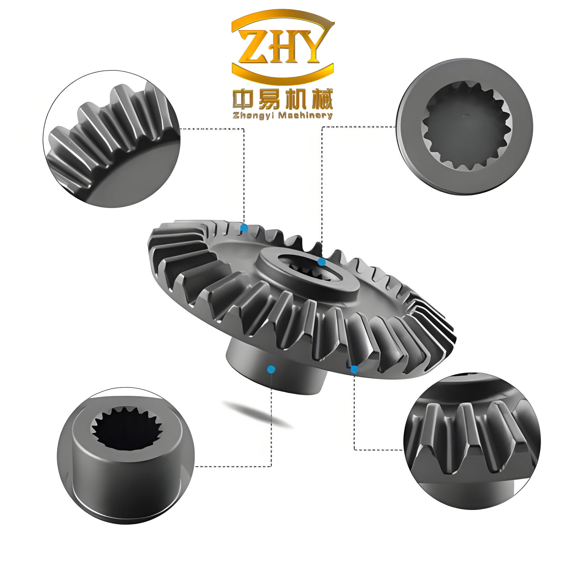
1. Why Straight Bevel Gears Matter in the Joint
Straight bevel gears transmit motion between intersecting shafts, usually at a shaft angle of 90 degrees. In my robotic joint, the straight bevel gears change the direction of the motor torque and allow the final axes to be packaged inside a narrow envelope. Compared with other bevel forms, straight bevel gears have teeth whose traces are straight and converge toward the cone apex. This geometry gives them a well-understood kinematic behavior, predictable manufacturing routes, and a relatively simple relationship between the pitch cone, root cone, and face cone. However, the same geometry also makes precise modeling more delicate than that of spur or helical gears because the tooth profile lies on a spherical surface rather than on a plane.
For my study, the main requirements for the straight bevel gears are:
1. The gear pair must have a one-to-one ratio because it only redirects power and does not change speed. 2. The tooth flanks must be generated from the spherical involute rather than from an approximate planar profile. 3. The model must be parametric so that module, tooth number, face width, pressure angle, and cone angle can be changed without rebuilding the entire feature tree. 4. The assembled straight bevel gears must show zero global interference. 5. The dynamic simulation must reproduce the theoretical ratio and reveal the influence of contact compliance and load direction. 6. The finite element analysis must expose the contact stress distribution along the tooth width and through the meshing cycle.
These requirements shape every later decision. I compare the common modeling routes for straight bevel gears, choose the spherical involute route, construct the tooth surfaces from equations and boundary curves, convert them into solids, assemble the full train, and then use multi-body dynamics and explicit finite element analysis to validate the design.
2. Modeling Routes for Straight Bevel Gears
I compare three families of methods that are commonly used for straight bevel gears. The first is the back-cone approximation. The second is machining simulation. The third is direct generation from the spherical involute theory. Each has a different balance of geometric accuracy, implementation effort, and parameter control.
| Method | Core Idea | Accuracy for Straight Bevel Gears | Parameter Control | Implementation Difficulty |
|---|---|---|---|---|
| Back-cone approximation | Unroll the back cone, draw a planar involute, and map or bend it onto a cone | Moderate; error grows when the spherical radius is small relative to the module | Good for standard designs | Low to moderate |
| Machining simulation | Model the cutter, workpiece, and machine kinematics, then generate the tooth surface by simulation | High when the actual cutting process is reproduced | Strong but dependent on machine settings | High |
| Spherical involute generation | Use the spherical involute equations directly to create tooth flank curves and surfaces | High; matches the theoretical tooth surface of straight bevel gears | Excellent when linked to parameter relations | Moderate |
I select the spherical involute generation method because it offers the best compromise for my application. It avoids the geometric approximation of the back-cone method, and it is more direct than a full machining simulation. The spherical involute also gives me a clean mathematical basis for parameterization. Once I encode the equations and relationships, I can change the module, tooth count, pressure angle, and cone angle and regenerate the straight bevel gears in a controlled way.
3. Spherical Involute Geometry of Straight Bevel Gears
The tooth profile of an ideal straight bevel gear is a spherical involute. I imagine a plane rolling without slipping on a base cone. A point on the plane traces a spherical curve on the sphere centered at the cone apex. That curve is the spherical involute. Because the surface is spherical, the usual planar involute equations do not apply directly. The spherical involute can be expressed in Cartesian coordinates as a function of the cone distance, the base cone angle, and the rolling angle.
Let $$l$$ be the cone distance, $$\theta$$ the base cone angle, and $$\phi$$ the rolling angle. The auxiliary angle $$\psi$$ is related to the rolling angle and the base cone angle. I use the following parametric form for the spherical involute of the straight bevel gear tooth flank:
$$
\begin{aligned}
x &= l\left(\sin\phi\sin\psi + \cos\phi\cos\psi\sin\theta\right),\\
y &= l\left(-\cos\phi\sin\psi + \sin\phi\cos\psi\sin\theta\right),\\
z &= l\cos\psi\cos\theta.
\end{aligned}
$$
The geometric relation between the auxiliary angle and the rolling angle is:
$$
\psi = \phi \sin\theta.
$$
The base cone angle is obtained from the pressure angle and the pitch cone angle:
$$
\sin\theta = \cos\alpha \sin\delta,
$$
where $$\alpha$$ is the pressure angle and $$\delta$$ is the pitch cone angle. These three equations form the mathematical backbone of my precise model of the straight bevel gears. I use them to create the large-end and small-end spherical involutes, and then I use those curves as boundaries for the tooth flank surfaces.
For a straight bevel gear pair with equal tooth numbers and a 90-degree shaft angle, the pitch cone angles are:
$$
\delta_1 = \delta_2 = 45^\circ.
$$
The pitch cone distance, or cone distance, is:
$$
R_e = \frac{m z}{2\sin\delta},
$$
where $$m$$ is the large-end module and $$z$$ is the tooth number. The addendum, dedendum, addendum angle, dedendum angle, face cone angle, and root cone angle follow from the standard straight bevel gear relations:
$$
h_a = \left(h_a^* + x\right)m,
$$
$$
h_f = \left(h_a^* + c^* – x\right)m,
$$
$$
\theta_a = \arctan\left(\frac{h_a}{R_e}\right),
$$
$$
\theta_f = \arctan\left(\frac{h_f}{R_e}\right),
$$
$$
\delta_a = \delta + \theta_a,
$$
$$
\delta_f = \delta – \theta_f.
$$
Here $$h_a^*$$ is the addendum coefficient, $$c^*$$ is the clearance coefficient, and $$x$$ is the profile shift coefficient. In my design, the straight bevel gears are standard, so the profile shift is zero. The pressure angle is 20 degrees. The module and tooth count are selected to satisfy the torque and packaging requirements.
4. Parametric Model Construction for Straight Bevel Gears
I build the straight bevel gears in a parametric CAD environment using a feature-based sequence. The key idea is to define a small set of primary parameters, then derive every other dimension through relations. This makes the straight bevel gears easy to update and keeps the tooth geometry consistent when the design changes.
4.1 Primary Parameters and Derived Relations
The primary parameters for the first straight bevel gear pair are listed below. I use the same structure for the second pair and for the additional gear pair that drives the second output axis.
| Parameter | Symbol | Value | Unit | Description |
|---|---|---|---|---|
| Large-end module | $$m$$ | 1.75 | mm | Module at the large end of the straight bevel gears |
| Tooth number | $$z$$ | 35 | – | Number of teeth on each gear of the pair |
| Face width | $$b$$ | 8 | mm | Width of the tooth along the cone distance |
| Pressure angle | $$\alpha$$ | 20 | degree | Standard pressure angle |
| Pitch cone angle | $$\delta$$ | 45 | degree | Equal cone angle for a one-to-one straight bevel gear pair |
| Addendum coefficient | $$h_a^*$$ | 1 | – | Standard addendum coefficient |
| Clearance coefficient | $$c^*$$ | 0.2 | – | Standard bottom clearance coefficient |
| Profile shift | $$x$$ | 0 | – | No profile shift in this design |
The derived relations are encoded in the parameter table so that the straight bevel gears remain mathematically consistent. The following table summarizes the most important relations.
| Derived Quantity | Relation | Purpose |
|---|---|---|
| Base cone angle | $$\theta = \arcsin\left(\cos\alpha \sin\delta\right)$$ | Controls the spherical involute |
| Cone distance | $$R_e = \frac{m z}{2\sin\delta}$$ | Sets the large-end pitch radius on the cone |
| Addendum | $$h_a = \left(h_a^* + x\right)m$$ | Defines the face cone |
| Dedendum | $$h_f = \left(h_a^* + c^* – x\right)m$$ | Defines the root cone |
| Addendum angle | $$\theta_a = \arctan\left(\frac{h_a}{R_e}\right)$$ | Sets the face cone angle |
| Dedendum angle | $$\theta_f = \arctan\left(\frac{h_f}{R_e}\right)$$ | Sets the root cone angle |
| Face cone angle | $$\delta_a = \delta + \theta_a$$ | Bounds the tooth top |
| Root cone angle | $$\delta_f = \delta – \theta_f$$ | Bounds the tooth root |
4.2 Reference Curves for Straight Bevel Gears
I create the reference curves in the following order. First, I generate the large-end spherical involute using the equations above. Second, I generate the small-end spherical involute by scaling the cone distance from the large end to the small end. Third, I create the large-end and small-end addendum circles and dedendum circles on their respective spherical surfaces. Fourth, I create the large-end pitch circle. Fifth, I find the intersection between the pitch circle and the spherical involute. This intersection is a key reference point because it defines the pitch point on the tooth flank. Sixth, I create a line connecting the corresponding endpoints of the large-end and small-end involutes.
These curves are not independent decorations. They are the exact boundaries of the tooth flank and the tooth tip and root surfaces. Because they come from the spherical involute and the standard cone relations, the resulting straight bevel gears have a tooth form that is consistent with the theoretical generating process.
4.3 Surface and Solid Generation
I then build the tooth flank surface by using a boundary blend between the large-end and small-end spherical involutes. The second boundary direction is the line connecting the involute endpoints. This produces a ruled-like surface that follows the spherical involute on both ends. I create a datum plane through the pitch point and the gear axis, rotate it by one quarter of the angular pitch, and mirror the first flank surface to obtain the opposite flank of the same tooth. The angular pitch is:
$$
\Delta = \frac{360^\circ}{z}.
$$
I construct the addendum surface and the dedendum surface as surfaces of revolution around the gear axis. I trim the flank, addendum, and dedendum surfaces with each other to form a single tooth surface group. I close the two ends of the tooth surface group with boundary surfaces. I merge all surfaces and solidify them into a single tooth solid. I then create the gear blank by revolving a profile around the axis. I apply a variable-radius fillet at the tooth root to reduce stress concentration. Finally, I pattern the tooth solid around the axis with the number of instances tied to the tooth number parameter and the angular spacing tied to the angular pitch. This creates the complete straight bevel gear.
I repeat the same procedure with the appropriate parameters for the mating straight bevel gear. Because the pair is one-to-one and symmetric, the two gears of the first pair are geometrically similar, but I still keep separate parameter sets so that the model remains flexible.
5. Assembly, Parameterization, and Interference Check
After creating the individual straight bevel gears, I assemble the gear train. The assembly constraints are also parameterized. The axis-to-axis angle, the axial positioning, and the phase of the teeth are controlled by relations. I set the shaft angle to 90 degrees and align the pitch cone apexes. I adjust the tooth phase so that the straight bevel gears mesh correctly without tooth interference. I then run a global interference check. The result is zero interference for the complete assembly.
The following table lists the main assembly checks I perform for the straight bevel gear train.
| Check | Target | Result in My Model | Consequence |
|---|---|---|---|
| Pitch cone apex coincidence | Apexes coincide | Satisfied | Correct cone kinematics |
| Shaft angle | 90 degrees | Satisfied | Proper direction change |
| Tooth phase | No interference in mesh | Satisfied | Continuous contact |
| Global interference | Zero volumes | Zero interference | Assembly is geometrically valid |
| Parameter update | Regeneration succeeds | Satisfied | The model is reusable |
The zero-interference result is important because approximate tooth profiles often produce small but non-physical intersections near the root or tip. Those intersections can corrupt later contact simulations. By using the spherical involute for the straight bevel gears, I avoid this problem and obtain a clean starting geometry for dynamics and finite element analysis.
6. Dynamic Simulation of the Straight Bevel Gear Train
I transfer the assembled model into a multi-body dynamics environment. My aim is to check whether the straight bevel gears produce the expected speed ratio, how the contact force behaves during acceleration and load changes, and whether the two output axes follow the commanded motion. I define rotational joints on the gear shafts, contact forces between the meshing teeth, a driving motion on each input shaft, and a resisting torque on each output shaft.
6.1 Contact Model for Straight Bevel Gears
I model the tooth contact with an impact-based contact force. The normal contact force consists of an elastic term and a damping term. A common form is:
$$
F_n = K \delta^e + C \dot{\delta},
$$
where $$K$$ is the contact stiffness, $$\delta$$ is the penetration depth, $$e$$ is the force exponent, $$C$$ is the damping coefficient, and $$\dot{\delta}$$ is the penetration velocity. I also apply a friction force based on the normal force and a friction coefficient. For lubricated steel straight bevel gears, I use a low friction coefficient.
For the four straight bevel gear pairs in the train, I calculate or estimate the contact stiffness from the tooth geometry and material. The values I use are listed below. They differ slightly because the gear sizes and tooth numbers differ among the stages.
| Gear Pair | Contact Stiffness | Damping | Force Exponent | Penetration Depth | Static Friction | Dynamic Friction |
|---|---|---|---|---|---|---|
| Pair 1 | $$5.90 \times 10^5$$ N/mm | 100 N·s/mm | 2.2 | 0.1 mm | 0.08 | 0.05 |
| Pair 2 | $$4.98 \times 10^5$$ N/mm | 100 N·s/mm | 2.2 | 0.1 mm | 0.08 | 0.05 |
| Pair 3 | $$7.37 \times 10^5$$ N/mm | 100 N·s/mm | 2.2 | 0.1 mm | 0.08 | 0.05 |
| Pair 4 | $$4.98 \times 10^5$$ N/mm | 100 N·s/mm | 2.2 | 0.1 mm | 0.08 | 0.05 |
I use step functions for the input angular velocity and the output load so that the simulation does not start with a sudden jump. The first input shaft is driven with an angular velocity that rises smoothly to 120 degrees per second. The second input shaft is driven with an angular velocity that rises smoothly to 90 degrees per second. The output loads are applied in stages so that I can observe the response before and after the load is reversed.
| Signal | Expression | Interpretation |
|---|---|---|
| Input 1 angular velocity | $$\omega_1 = \mathrm{step}(t,0,0^\circ/\mathrm{s},0.5,120^\circ/\mathrm{s})$$ | Smooth ramp to 120 degrees per second |
| Output 1 torque | $$T_1 = \mathrm{step}(t,0,0,0.5,-200) + \mathrm{step}(t,1.5,0,2,200)$$ | Load then reverse load |
| Input 2 angular velocity | $$\omega_2 = \mathrm{step}(t,0,0^\circ/\mathrm{s},0.5,90^\circ/\mathrm{s})$$ | Smooth ramp to 90 degrees per second |
| Output 2 torque | $$T_2 = \mathrm{step}(t,0,0,0.5,100) + \mathrm{step}(t,1.5,0,2,-100)$$ | Load then reverse load |
6.2 Dynamic Results for the Straight Bevel Gears
I run the simulation with a short time step and record the angular velocities of the input and output shafts. The first output axis is driven directly by a straight bevel gear pair, so its speed should equal the input speed after the ramp. The second output axis passes through an additional spur gear stage and another straight bevel gear pair, so it has a different theoretical ratio. I compare the average simulated speeds with the theoretical values.
| Output Axis | Simulated Average Speed | Theoretical Average Speed | Relative Error |
|---|---|---|---|
| Output axis 1 | 90.3765 degrees per second | 90.1052 degrees per second | 0.30 percent |
| Output axis 2 | 97.0769 degrees per second | 94.6106 degrees per second | 2.50 percent |
The first output axis follows the theoretical speed of the straight bevel gears very closely. The small fluctuation around the mean comes from the discrete tooth contact and the compliance of the contact model. The second output axis shows a larger error because the power passes through more stages. The additional spur gear pair and the second straight bevel gear pair accumulate contact compliance, backlash, and numerical damping. Even so, the average speed is close enough to the theoretical value to confirm that the overall transmission concept and the straight bevel gear modeling are correct.
The dynamic simulation also shows that the contact force is intermittent. Each tooth pair engages, carries load, and separates. The force magnitude depends on the applied torque, the contact stiffness, and the angular position. When the load reverses, the contact switches to the opposite flank of the straight bevel gears. This behavior is consistent with the expected backlash and contact geometry.
7. Finite Element Analysis of the Straight Bevel Gear Contact
After the dynamic simulation, I examine the stress state of the most critical straight bevel gear pair. I use a dedicated preprocessor for mesh generation and an explicit finite element solver for the contact calculation. The goal is not only to obtain a maximum stress value but also to understand how the contact stress moves across the tooth surface during meshing.
7.1 Mesh Strategy for Straight Bevel Gears
I use a mixed mesh strategy. The teeth that are expected to enter contact are meshed with fine hexahedral elements. The rest of the gear is meshed with coarser tetrahedral elements. This reduces the computational cost while preserving accuracy in the contact zone. I separate the model into a contact tooth group and a non-contact body group. The two groups are connected with tie constraints.
| Region | Element Type | Mesh Density | Reason |
|---|---|---|---|
| Contact teeth | C3D8R hexahedral | Fine | Accurate contact stress and tooth bending |
| Non-contact body | C3D10M tetrahedral | Coarse | Reduce degrees of freedom |
| Connection | Tie constraint | – | Transfer displacement between regions |
| Boundary coupling | Rigid reference point | – | Apply rotation and torque |
I model seven teeth as the contact group. This number is large enough to include the actual contact zone and the neighboring teeth that share load, but it is small enough to keep the explicit analysis practical. I apply a rotating velocity to the reference point of the driving straight bevel gear and a resisting torque to the reference point of the driven straight bevel gear. The shaft holes are coupled to the reference points so that the motion and load enter the gear body in a realistic way.
7.2 Contact Formulation and Material Assumptions
For the finite element contact, I use a hard normal contact and a penalty friction formulation. The normal contact pressure is approximated as a function of penetration:
$$
p_n =
\begin{cases}
K_n g^m, & g > 0,\\
0, & g \le 0,
\end{cases}
$$
where $$g$$ is the penetration, $$K_n$$ is the normal contact stiffness, and $$m$$ is the pressure exponent. The frictional shear stress is limited by:
$$
\tau_f \le \mu p_n,
$$
where $$\mu$$ is the friction coefficient. The material is assumed to be linear elastic steel with the following properties.
| Property | Value | Unit |
|---|---|---|
| Elastic modulus | 210 | GPa |
| Poisson ratio | 0.30 | – |
| Density | 7850 | kg/m³ |
| Friction coefficient | 0.05 | – |
7.3 Stress Evolution in the Straight Bevel Gears
The explicit analysis produces a sequence of stress fields. At the beginning, the stress concentrates near the shaft hole because the velocity and torque are applied through the rigid reference point. As the teeth come into contact, the stress moves to the contacting flanks. The contact region then travels along the tooth surface as the gears rotate. The highest stress appears near the mid-to-large end of the tooth, where the tooth stiffness is higher and the load is transferred across the face width.
I track a single node on the active flank of a driving straight bevel gear. Its normal contact stress rises when the tooth enters mesh, remains nonzero during the contact period, and falls to zero when the tooth leaves mesh. This confirms that the contact is not continuous at a fixed point but moves across the tooth surface. I also extract a series of nodes along a path from the small end to the large end of the same tooth. The stress distribution along that path is relatively flat in the middle and drops at both ends. The middle region carries a fairly uniform contact pressure, while the ends show local peaks that indicate the need for edge relief or tooth crowning.
| Observation | Physical Meaning | Design Implication |
|---|---|---|
| Stress starts at the shaft hole | Load introduction through the coupling point | Check hub and shaft fit |
| Stress moves to the tooth flank | Contact develops between meshing straight bevel gears | Focus on tooth flank quality |
| Stress travels along the tooth | Meshing progresses from root to tip and across the face | Check contact ratio and alignment |
| Mid-face stress is uniform | The central part of the tooth shares load well | The basic geometry is sound |
| End stress peaks | Edge contact concentration | Apply edge relief or crowning |
8. Interpretation of the Simulation Results
The dynamic and finite element results support each other. The dynamic simulation shows that the straight bevel gears transmit the commanded motion with an average speed ratio close to the theoretical value. The small velocity fluctuations are consistent with the periodic engagement and disengagement of the teeth. The finite element analysis shows that the contact stress is concentrated on the active flanks and that the stress path moves with the mesh. The stress distribution along the tooth width has a plateau in the middle and peaks near the ends. This is a common pattern for straight bevel gears and indicates that the basic tooth form is correct but that edge modification could improve durability.
I also examine the sensitivity of the results to some key parameters. The contact stiffness affects the amplitude and duration of the contact force. A higher stiffness produces a shorter, sharper contact impulse. The friction coefficient affects the tangential force and the heat generation, but its influence on the normal contact stress is smaller under the investigated loads. The face width affects the load distribution along the tooth. A wider face can reduce the average contact pressure, but if the alignment is imperfect, it can also increase the edge stress. The pressure angle affects the tooth thickness and the contact ratio. A larger pressure angle generally increases the tooth root thickness but also changes the contact position on the spherical involute.
| Parameter | Effect on Straight Bevel Gears | Practical Consideration |
|---|---|---|
| Module | Controls tooth size and contact stiffness | Larger module increases load capacity but reduces compactness |
| Tooth number | Controls angular pitch and contact ratio | More teeth smooth the motion but reduce tooth size for a given cone distance |
| Face width | Controls load distribution along the tooth | Wider face helps only with good alignment |
| Pressure angle | Controls tooth shape and root strength | Standard 20 degrees is a good compromise |
| Profile shift | Controls tooth thickness and undercut | Useful for avoiding undercut in small tooth counts |
| Root fillet | Controls stress concentration | Variable-radius fillet improves fatigue life |
9. Parametric Relationships and Numerical Checks
To make the straight bevel gear model useful for further design, I keep all important dimensions linked by equations. The following relationships are the ones I check most often.
The angular pitch of the straight bevel gears is:
$$
\Delta = \frac{360^\circ}{z}.
$$
The pitch cone radius at the large end is:
$$
r_e = \frac{m z}{2}.
$$
The pitch cone distance is:
$$
R_e = \frac{r_e}{\sin\delta}.
$$
The face width should normally satisfy:
$$
b \le \frac{R_e}{3}.
$$
In my design, $$R_e$$ is approximately 43.3 mm and $$b$$ is 8 mm, so the face width is well within the recommended range. The contact ratio of the straight bevel gears is influenced by the tooth height and the pressure angle. I do not need to calculate it analytically at every step because the contact simulation captures the actual contact behavior, but the geometric ratio remains a useful sanity check.
The transmission ratio of a straight bevel gear pair is:
$$
i = \frac{\omega_1}{\omega_2} = \frac{z_2}{z_1}.
$$
For the first pair, $$z_1 = z_2 = 35$$, so $$i = 1$$. For the second output path, the additional spur gear stage changes the total ratio. The theoretical output speed of the second axis is therefore not equal to the input speed of the second motor. This is why I compare each output axis with its own theoretical value rather than with a single global ratio.
10. Contact Force and Stress Estimates
I also use simplified estimates to check the finite element results. For a straight bevel gear tooth, the normal force can be related to the torque by the pitch radius and the pressure angle. If $$T$$ is the torque on the gear and $$r_m$$ is the mean pitch radius, the tangential force is approximately:
$$
F_t = \frac{T}{r_m}.
$$
The normal force on the tooth flank is then:
$$
F_n = \frac{F_t}{\cos\alpha}.
$$
The radial and axial components follow from the cone angle and the pressure angle. For a 90-degree straight bevel gear pair with equal cone angles, the axial force on one gear is equal in magnitude to the radial force on the mating gear. These force components are useful because they determine the bearing loads and the shaft deflections. If the shaft deflection is too large, the contact pattern shifts toward the tooth ends and the edge stress increases. The finite element analysis shows exactly this tendency as local peaks near the small and large ends.
| Quantity | Formula | Role in Straight Bevel Gear Design |
|---|---|---|
| Tangential force | $$F_t = \frac{T}{r_m}$$ | Drives tooth bending and contact load |
| Normal force | $$F_n = \frac{F_t}{\cos\alpha}$$ | Controls contact pressure |
| Radial force | $$F_r = F_t \tan\alpha \cos\delta$$ | Loads the bearings |
| Axial force | $$F_a = F_t \tan\alpha \sin\delta$$ | Loads the thrust bearings |
| Mean pitch radius | $$r_m = R_e – 0.5b \sin\delta$$ | Used for force estimation |
These estimates are approximate, but they help me interpret the finite element output. The maximum contact stress should be on the order of the elastic contact stress for steel under the applied normal load. If the simulated stress is much lower, the contact may not be fully developed. If it is much higher, there may be an edge concentration or an artificial numerical peak.
11. Modeling Quality and Validation
I validate the model in several ways. First, the geometry check confirms zero interference. Second, the dynamic simulation confirms the expected speed ratio. Third, the finite element analysis produces a contact stress pattern that is physically reasonable for straight bevel gears. Fourth, the parameter changes propagate correctly through the model. When I change the module or tooth number, the spherical involute, cone angles, tooth thickness, and pattern spacing all update consistently.
| Validation Item | Method | Result |
|---|---|---|
| Tooth surface accuracy | Spherical involute equations | High |
| Assembly fit | Global interference check | Zero interference |
| Kinematic ratio | Multi-body dynamics | Close to theoretical |
| Contact stress | Explicit finite element analysis | Reasonable distribution |
| Parameter update | Parametric regeneration | Successful |
The validation also reveals limitations. The contact stiffness in the multi-body model is a lumped parameter, so it cannot reproduce the detailed stress field. The finite element model uses a linear elastic material, so it does not capture plasticity or fatigue. The friction coefficient is assumed constant, while in reality it depends on speed, temperature, and lubrication. These limitations are acceptable for my current purpose because I am comparing design alternatives rather than predicting absolute life. For a final production design, I would refine the contact model, include thermal effects, and use measured surface finish and lubrication data.
12. Design Improvements Suggested by the Analysis
The analysis suggests several improvements for the straight bevel gears. The most important is edge relief. The stress peaks near the small and large ends indicate that the tooth edges carry more load than the middle region under some alignment conditions. A small amount of crowning or edge rounding can spread the contact and reduce the peak stress. The second improvement is to increase the root fillet radius if the packaging allows it. A larger fillet reduces the bending stress concentration and improves fatigue life. The third improvement is to control the shaft stiffness. If the shafts deflect too much under load, the contact pattern moves toward one end of the tooth. Increasing the shaft diameter or reducing the overhang can improve the contact distribution.
| Improvement | Expected Benefit | Possible Cost |
|---|---|---|
| Tooth edge relief | Lower edge stress and smoother contact | Additional manufacturing step |
| Larger root fillet | Higher bending fatigue strength | May reduce usable tooth height |
| Stiffer shafts | Better contact alignment | More mass and space |
| Profile shift | Improved tooth thickness and undercut control | Requires retuning the spherical involute |
| Surface finish control | Lower friction and better contact | Higher manufacturing cost |
I would apply these improvements iteratively. First, I would modify the tooth edge geometry and rerun the finite element contact analysis. Second, I would adjust the root fillet and check the bending stress. Third, I would update the dynamic model with the new contact stiffness and verify that the speed ratio and contact force remain acceptable. This loop is efficient because the straight bevel gear model is parametric and the simulation workflow is already established.
13. Broader Use of the Workflow
The same workflow can be applied to other straight bevel gear systems. The key steps are always the same: define the primary parameters, derive the cone geometry, generate the spherical involute, build the tooth surfaces, solidify the tooth, pattern it around the axis, assemble the train, simulate the dynamics, and analyze the contact. The specific values change, but the logic remains. I can use this workflow for straight bevel gears with different modules, tooth numbers, pressure angles, and shaft angles. I can also extend it to straight bevel gears with profile shift or non-standard addendum coefficients.
For a robot joint, the workflow is especially useful because the packaging is tight and the load direction changes frequently. A precise model of the straight bevel gears helps me evaluate whether the joint can survive repeated forward and reverse motion. The dynamic simulation shows how the contact force changes when the load reverses, and the finite element analysis shows where the stress concentrates. Together, they give me a clear picture of the design margins.
14. Summary of Equations
For convenience, I collect the main equations used in my model of the straight bevel gears. These equations define the spherical involute, the cone geometry, the force components, and the contact behavior.
$$
\begin{aligned}
x &= l\left(\sin\phi\sin\psi + \cos\phi\cos\psi\sin\theta\right),\\
y &= l\left(-\cos\phi\sin\psi + \sin\phi\cos\psi\sin\theta\right),\\
z &= l\cos\psi\cos\theta,\\
\psi &= \phi \sin\theta,\\
\sin\theta &= \cos\alpha \sin\delta,\\
R_e &= \frac{m z}{2\sin\delta},\\
h_a &= \left(h_a^* + x\right)m,\\
h_f &= \left(h_a^* + c^* – x\right)m,\\
\theta_a &= \arctan\left(\frac{h_a}{R_e}\right),\\
\theta_f &= \arctan\left(\frac{h_f}{R_e}\right),\\
\delta_a &= \delta + \theta_a,\\
\delta_f &= \delta – \theta_f,\\
\Delta &= \frac{360^\circ}{z},\\
i &= \frac{z_2}{z_1},\\
F_t &= \frac{T}{r_m},\\
F_n &= \frac{F_t}{\cos\alpha},\\
F_r &= F_t \tan\alpha \cos\delta,\\
F_a &= F_t \tan\alpha \sin\delta.
\end{aligned}
$$
The contact force in the dynamic model is:
$$
F_n = K \delta^e + C \dot{\delta}.
$$
The normal contact pressure in the finite element model is:
$$
p_n =
\begin{cases}
K_n g^m, & g > 0,\\
0, & g \le 0.
\end{cases}
$$
The frictional shear limit is:
$$
\tau_f \le \mu p_n.
$$
15. Conclusions from My Modeling and Simulation
I have completed a precise parametric model of a straight bevel gear train and used it for dynamic and finite element analysis. The main conclusions are as follows.
First, the spherical involute method is the most suitable route for precise modeling of straight bevel gears in this application. It gives a tooth surface that matches the theoretical generating geometry and avoids the approximation error of the back-cone method. The resulting straight bevel gears assemble with zero interference.
Second, the parametric relations allow the straight bevel gears to be updated quickly. Module, tooth number, face width, pressure angle, and cone angle can all be changed while the tooth surfaces, cone angles, and pattern spacing update consistently.
Third, the dynamic simulation confirms that the straight bevel gear train transmits motion with the expected speed ratio. The first output axis follows the input speed closely. The second output axis has a larger but acceptable error because it includes additional transmission stages.
Fourth, the finite element contact analysis shows a moving contact zone and a stress distribution that is reasonable for straight bevel gears. The stress is relatively uniform in the middle of the tooth and rises near the ends, which suggests that edge relief or crowning would improve the contact.
Fifth, the combined use of parametric CAD, multi-body dynamics, and explicit finite element analysis provides a practical workflow for straight bevel gear design. I can use the same workflow to study other straight bevel gears, optimize the tooth geometry, and improve the durability of the robotic joint.
Overall, the model and simulations give me confidence that the straight bevel gears in the joint can perform the required motion and carry the required load. The remaining work is to refine the edge geometry, verify the manufacturing tolerances, and include more detailed lubrication and thermal effects in the contact model. Because the straight bevel gear model is parametric and the simulation pipeline is established, those refinements can be made without rebuilding the entire study.