
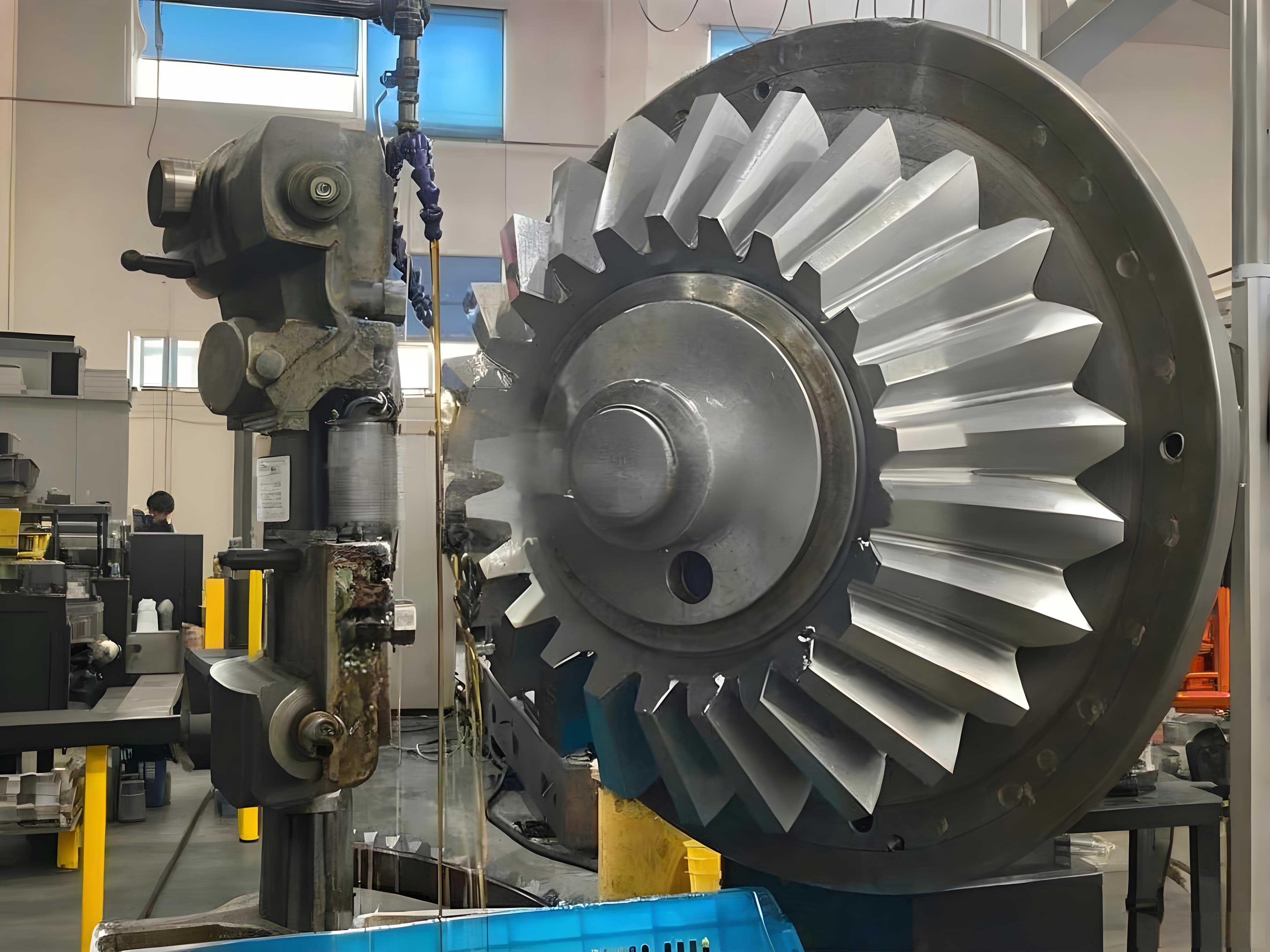
In the realm of power transmission, particularly in applications requiring efficient 90-degree shaft redirection, miter gears—a specific subset of straight bevel gears with a 1:1 ratio—hold significant importance. The traditional paradigm for evaluating the design and quality of these components has long relied on theoretical tooth contact analysis (TCA) simulations and physical rolling tests. However, a fundamental discrepancy exists between these two pillars. Theoretical TCA operates on a perfect, idealized geometry, while physical rolling tests are conducted on manufactured parts that inevitably contain machining errors. This creates a disconnect between the design benchmark and the inspection standard. Furthermore, physical rolling tests are often cumbersome, requiring tedious machine setup and adjustments, and are susceptible to significant experimental error themselves.
A compelling solution to this challenge is the concept of a “digital twin” for the gear tooth surface. By constructing a highly accurate mathematical model that faithfully represents the actual, manufactured tooth surface, one can bridge the gap between design and reality. This digital representation can then be used for precise digital TCA, simulating meshing performance based on the real geometry, and can even facilitate a new form of digital roll testing, eliminating the need for physical prototypes in the debugging phase. Researchers have explored various avenues for this reconstruction. Some have proposed representing the real surface by superimposing a theoretical surface with an error surface defined by complex nonlinear equations. Others have employed uniform bicubic B-spline surfaces to fit coordinate measurement machine (CMM) data, creating a mathematical expression for the deviation field. Interpolation B-spline surfaces have also been applied. While these methods mark important progress, they can sometimes suffer from relatively large fitting errors or offer limited control over the final shape of the reconstructed surface.
Building upon this foundation, this work proposes the application of Non-Uniform Rational B-Splines (NURBS) for fitting the tooth surfaces of straight bevel and miter gears. The unique advantage of NURBS lies in its incorporation of weight factors alongside control points and knot vectors. These weight factors provide an additional degree of freedom, allowing for superior local shape control, which is crucial for accurately capturing the nuanced geometry of a gear tooth, including potential modifications or wear patterns. This capability often leads to higher fitting accuracy with fewer control points compared to standard B-splines. The versatility and power of NURBS have made it the industry standard, formally recognized by the International Organization for Standardization (ISO) as the sole mathematical method for representing free-form curves and surfaces, and it is ubiquitous in aerospace, automotive, and shipbuilding CAD/CAM systems. Therefore, investigating the use of NURBS for fitting miter gear tooth surfaces is both practically relevant and theoretically sound.
The mathematical journey begins with the NURBS curve, which forms the building block for surfaces. A p-th degree NURBS curve is defined by:
$$
\mathbf{C}(u) = \frac{\sum_{i=0}^{n} w_i N_{i,p}(u) \mathbf{P}_i}{\sum_{i=0}^{n} w_i N_{i,p}(u)}
$$
where:
- $\mathbf{P}_i$ are the control points forming a polygon that approximates the curve’s shape.
- $w_i$ are the corresponding weights. When all weights are equal, the NURBS curve reduces to a standard B-spline.
- $N_{i,p}(u)$ are the p-th degree B-spline basis functions, defined recursively on a non-uniform knot vector $\mathbf{U} = \{u_0, u_1, …, u_{m}\}$.
- The parameter $u$ varies within the interval $[u_p, u_{n+1}]$.
For the specific and common case of a cubic (degree p=3) NURBS curve, the basis functions can be efficiently evaluated. More importantly for interpolation, the curve segment between two distinct knots can be expressed in matrix form. This is particularly useful for computational efficiency. Given a normalized local parameter $t \in [0, 1]$ for a segment defined by knots $u_i$ to $u_{i+1}$, the curve can be written as:
$$
\mathbf{C}_i(t) = \frac{ \mathbf{T} \cdot \mathbf{M} \cdot \mathbf{G}_w }{ \mathbf{T} \cdot \mathbf{M} \cdot \mathbf{W} }
$$
where $\mathbf{T} = [t^3, t^2, t, 1]$, $\mathbf{M}$ is the constant cubic B-spline basis matrix, $\mathbf{G}_w$ is the geometric vector of weighted control points $[w_i\mathbf{P}_i, w_{i+1}\mathbf{P}_{i+1}, w_{i+2}\mathbf{P}_{i+2}, w_{i+3}\mathbf{P}_{i+3}]^T$, and $\mathbf{W}$ is the weight vector $[w_i, w_{i+1}, w_{i+2}, w_{i+3}]^T$.
The core task in reconstruction is interpolation: given a set of measured data points $\mathbf{Q}_k$ (the “type值点” or sample points) on the actual miter gear tooth surface, we must find a NURBS curve (and later, surface) that passes exactly through them. This is an inverse problem: we know the data points and need to solve for the unknown control points $\mathbf{P}_i$ and, optionally, optimal weights $w_i$.
The process involves several key steps:
- Parameterization: Each data point $\mathbf{Q}_k$ must be assigned a parameter value $\bar{u}_k$ along the curve’s domain. A robust and commonly used method is cumulative chord length parameterization, which accounts for the geometric spacing of points:
$$
\bar{u}_0 = 0, \quad \bar{u}_k = \bar{u}_{k-1} + \frac{||\mathbf{Q}_k – \mathbf{Q}_{k-1}||}{L}, \quad L = \sum_{j=1}^{n} ||\mathbf{Q}_j – \mathbf{Q}_{j-1}||
$$
This typically produces better results than uniform parameterization, especially for unevenly spaced points. - Knot Vector Generation: A corresponding knot vector $\mathbf{U}$ must be chosen. For interpolation, a common approach is to average the parameter values of the internal data points. For a cubic curve interpolating $n+1$ points, the knot vector has $n+7$ knots, with the first and last four knots clamped (e.g., $\{0,0,0,0, \bar{u}_1, \bar{u}_2, …, \bar{u}_{n-1}, 1,1,1,1\}$).
- Setting Up the Linear System: The interpolation condition $\mathbf{C}(\bar{u}_k) = \mathbf{Q}_k$ for all $k$ leads to a system of linear equations. Assuming initially that all weights $w_i = 1$ (simplifying to a B-spline interpolation first), the equation for the $k$-th data point becomes:
$$
\sum_{i=0}^{n} N_{i,3}(\bar{u}_k) \mathbf{P}_i = \mathbf{Q}_k
$$
This forms a linear system $\mathbf{N} \cdot \mathbf{P} = \mathbf{Q}$, where $\mathbf{N}$ is a matrix of basis function values evaluated at the parameter $\bar{u}_k$. - Applying Boundary Conditions: The system $\mathbf{N} \cdot \mathbf{P} = \mathbf{Q}$ has $n+1$ equations but $n+3$ unknown control points for a clamped cubic curve. Two additional equations are needed, which come from specifying end conditions. The most physically meaningful for a miter gear tooth profile are the endpoint derivative conditions (clamped boundary). We can prescribe the first derivatives (tangent vectors) at the start and end of the curve, $\mathbf{D}_0$ and $\mathbf{D}_n$. For a cubic NURBS curve with clamped knots, these derivatives are:
$$
\mathbf{C}'(0) = \frac{3}{u_{4}-u_{3}} \frac{w_1}{w_0} (\mathbf{P}_1 – \mathbf{P}_0), \quad \mathbf{C}'(1) = \frac{3}{u_{n+3}-u_{n+2}} \frac{w_{n+1}}{w_{n+2}} (\mathbf{P}_{n+2} – \mathbf{P}_{n+1})
$$
With weights initially set to 1, these simplify to equations involving the first two and last two control points. Adding these two equations to the system yields a solable $(n+3) \times (n+3)$ linear system.
| Parameter | Pinion | Gear (Miter Mate) |
|---|---|---|
| Number of Teeth, \(z\) | 16 | 16 |
| Module, \(m_n\) (mm) | 4.0 | 4.0 |
| Pressure Angle, \(\alpha\) (°) | 20 | 20 |
| Shaft Angle, \(\Sigma\) (°) | 90 | 90 |
| Face Width, \(b\) (mm) | 20 | 20 |
| Pitch Cone Distance, \(R\) (mm) | 90.51 | 90.51 |
| Addendum, \(h_a\) (mm) | 4.0 | 4.0 |
| Dedendum, \(h_f\) (mm) | 4.8 | 4.8 |
To extend this from curves to surfaces for a complete miter gear tooth, we employ a tensor-product NURBS surface. A biparametric NURBS surface of degree p in the u direction and degree q in the v direction is defined as:
$$
\mathbf{S}(u,v) = \frac{\sum_{i=0}^{n} \sum_{j=0}^{m} w_{i,j} N_{i,p}(u) N_{j,q}(v) \mathbf{P}_{i,j}}{\sum_{i=0}^{n} \sum_{j=0}^{m} w_{i,j} N_{i,p}(u) N_{j,q}(v)}
$$
The fitting process is fundamentally a two-stage interpolation:
- First, we organize the measured 3D point cloud from the CMM into a grid structure, with points arranged along roughly orthogonal directions on the tooth surface (e.g., profile direction and lead direction). One direction is designated as the u direction. For each fixed row of points in the v direction, we perform a cubic NURBS curve interpolation (as described above) along the u direction. This gives us a set of intermediate control points for each curve.
- Second, these intermediate control points are now treated as new “data points” arranged in the v direction. For each column of these points, we perform another cubic NURBS curve interpolation, this time along the v direction. The final result of this step yields the full bidirectional grid of control points \(\mathbf{P}_{i,j}\) for the surface.
This method, known as global surface interpolation, ensures the fitted NURBS surface passes through all the original measured grid points. The density and distribution of the initial data points are critical. A finer grid captures more detail but increases computation time. For a miter gear tooth, a non-uniform grid, denser in regions of high curvature (like the fillet and active profile near the pitch line), is advisable.
The quality of the fitted NURBS surface for the miter gears is quantified through error analysis. The primary metric is the geometric deviation between the original measured points \(\mathbf{Q}_{k,l}\) and their corresponding closest points on the fitted NURBS surface \(\mathbf{S}(u_k, v_l)\). For a perfect interpolation, this deviation is zero. However, in practice, due to numerical rounding and the specifics of knot placement, minor deviations exist. A more rigorous check involves calculating the normal projection error for a denser set of validation points not used in the interpolation.
The error at any given point can be found by solving a minimization problem. For a validation point \(\mathbf{V} = (X, Y, Z)\), we find the parameters \((\hat{u}, \hat{v})\) that minimize the distance to the surface \(\mathbf{S}(u,v)\):
$$
\min F(u,v) = ||\mathbf{S}(u,v) – \mathbf{V}||^2
$$
This is typically solved using iterative methods like Newton-Raphson, starting from a good initial guess. The fitting error \(E\) is then this minimum distance. By calculating \(E\) for a dense cloud of validation points across the entire tooth flank of the miter gear, we can compute statistics such as the maximum error (\(E_{max}\)), root-mean-square error (\(E_{RMS}\)), and mean error.
| Factor | Influence on NURBS Fitting | Recommendation for Miter Gears |
|---|---|---|
| Data Point Density | Higher density improves accuracy but increases system size and computation time. Essential in high-curvature zones. | Use adaptive sampling: denser near root, pitch line, and edges; sparser on flatter regions of the flank. |
| Parameterization Method | Affects parameter distribution. Uniform can cause loops/flats; chord-length or centripetal is generally better. | Use cumulative chord length for geometric point sets from CMM scans of the miter gear tooth. |
| Knot Vector Placement | Determines basis function support and curve flexibility. Averaging interior parameters is standard for interpolation. | Use knot placement based on averaged parameter values from chord-length parameterization. |
| Boundary Conditions | Clamped end derivatives strongly influence edge behavior. Accurate tangent info at edges improves overall fit. | Estimate end tangents from the first and last few measured points on the miter gear tooth profile/lead. |
| Weight Factors (\(w_{i,j}\)) | Provide extra shape control. Defaulting to 1 is common; optimization can improve conic section representation. | Start with all weights = 1. Optimize only if specific known conical features on the miter gear need exact representation. |
Let’s consider a practical error assessment. Suppose we have interpolated a NURBS surface for a miter gear pinion using a 9×5 grid of measured points (9 points along the profile, 5 along the lead). After fitting, we evaluate errors at the original 45 points and at an additional 200 randomly distributed validation points on the tooth. A hypothetical error summary might show:
$$
E_{max, interpolated} \approx 5 \times 10^{-4} \text{ mm}, \quad E_{RMS, validation} \approx 2 \times 10^{-4} \text{ mm}
$$
These errors are on the order of sub-microns to a few microns, which is well within acceptable tolerances for high-precision miter gear applications. This confirms that the NURBS-fitted surface is a highly accurate digital representation of the physical tooth, capable of replacing it for digital simulation purposes.
The mathematical model of the tooth surface, now encoded as a NURBS entity \(\mathbf{S}(u,v)\), unlocks powerful digital workflows. It can be directly used in advanced TCA software to simulate the meshing and contact patterns under load with the actual gear geometry, providing insights into transmission error, stress distribution, and noise generation. Furthermore, this exact digital model can be fed into CNC machining centers to guide manufacturing or re-manufacturing processes, ensuring consistency. Most significantly, it enables the concept of digital roll testing. The digital models of a mating pair of miter gears can be virtually “rolled” together in software, analyzing their kinematic and dynamic interaction without ever cutting metal. This allows for rapid design iteration, tolerance analysis, and performance prediction, dramatically reducing development time and cost for systems employing miter gears.
In conclusion, the application of NURBS surface interpolation for reconstructing straight bevel and miter gear tooth surfaces presents a robust and high-fidelity methodology. By leveraging its superior shape control through weights and its status as an industry standard, NURBS provides a mathematically sound basis for creating a digital twin of the physical gear. The process, involving careful parameterization, knot vector generation, and the solution of linear systems with appropriate boundary conditions, yields surfaces with micron-level accuracy. This accuracy validates the use of the fitted NURBS surface as a substitute for the real tooth in analytical and digital validation processes. The transition from this digital model to digital tooth contact analysis and fully virtual roll testing represents a paradigm shift in gear design and quality assurance, offering unprecedented precision, efficiency, and insight for the engineering of power transmission systems, especially those utilizing critical 90-degree power transfer components like miter gears.