
In this research, I investigate the surface roughness prediction of spiral bevel gears machined on a CNC milling center. Large-size spiral bevel gears are critical components in high-power transmission systems, especially in thermal power generation, marine propulsion, wind turbines, and aerospace power transmission. The continuous demand for energy has led to an increasing need for large spiral bevel gears and their assemblies. Traditionally, these gears are manufactured using dedicated gear cutting machines, such as gear hobbing machines with peripheral cutting, continuous generating spiral hobbing, and conical-type cutting. However, the emergence of multi-task or multi-process machines, along with continuous improvements in numerical control and CAM software, has created a suitable medium for manufacturing these complex geometric elements using standard general-purpose machines and tools. This technology is particularly suitable for high-module gears with modules ranging from 4 mm to 12 mm. The use of standard tools also offers advantages in reducing costs and delivery time, which are critical parameters in production. To provide flexible options, small or medium batches of large spiral bevel gears are produced using 5-axis machine tools and disc cutter cutting methods. This approach also allows the manufacture of various gear geometries, such as straight gears, helical gears, double helical gears, bevel gears, and hypoid gears. Gear manufacturing in multi-task machines is seen as an increasingly broad solution, especially considering their high flexibility. Both 4-axis and 5-axis CNC machining can be used for the manufacture of spiral bevel gears. The advantages of this method include increased versatility of the manufacturing process, both in terms of type and size, and the ability to achieve arbitrary modifications of different gear teeth. To ensure the quality of manufactured parts and gear contact, special attention must be paid to the machining process of the gear surfaces.
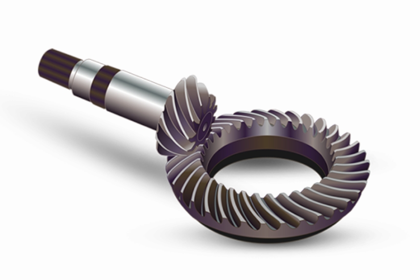
I design a multi-process milling machine prediction model for the surface roughness of spiral bevel gears. This model estimates the surface topography of each gear surface based on parameters such as tool tilt angle and direction, geometric cutting parameters, milling cutter feed, and rotational speed. Through different machining conditions, I optimize the gear finishing process. Therefore, there is no need to perform trial-and-error tests, which saves cost and time. This optimization process also allows the adjustment of cutting parameters according to the required surface quality without machining more channels, which also reduces machining time and tool life.
The developed model estimates the spiral bevel gear tooth surface topography depending on machining parameters such as tool tilt angle and direction, cutting geometric parameters, and tool feed and speed values. I tested the model with two different finishing operations: a 5-axis machining operation and a 3+2-axis machining operation, to determine the effect of the number of machining axes on surface finish. The gap trajectory between indexing teeth is represented in the model. In the first step, for each interpolation point, the model obtains the machining program (CL data): tool tip point position \((x_j, y_j, z_j)\) and the defined tool axis orientation direction vector \((u_j, v_j, w_j)\) in the workpiece reference system \(X, Y, Z\). The milling trajectory can be obtained from the coordinates of consecutive tool tip points. After eliminating the initial and final non-cutting motions, I evaluate the milling trajectory. In the feed direction, I define five simulation regions. Each simulation region is defined by six points in the feed direction and approximately thirty points in the direction perpendicular to the feed direction. The size of the simulation region depends on the programmer’s standard. Then, I predict the surface topography generated by each simulation region. To achieve this, I define a local reference system \(O_W X_W Y_W Z_W\) for each simulation region. First, I derive the position of the tool center point \(C\) of the selected simulation region.
To predict the surface topography generated by each simulation region, I define a local coordinate system \(O_W X_W Y_W Z_W\) attached to the workpiece (spiral bevel gear tooth surface). The definition of the local coordinate system for each simulation region is based on the tool tip point position and the tool axis direction given in the machining program of the reference milling trajectory. The origin \(O_W\) and axis \(Z_W\) are the first system elements obtained. To achieve this, I consider a set of auxiliary elements: a point \(M\) and two unit vectors \(\hat{u}\) and \(\hat{q}\). First, I select two interpolation points \(A\) and \(B\) at the center of the reference trajectory and consider the midpoint \(D\) of the linear interpolation between points \(A\) and \(B\). The coordinates of point \(D\) \((x_D, y_D, z_D)\) are functions of the coordinates of points \(A\) and \(B\) \((x_A, y_A, z_A)\) and \((x_B, y_B, z_B)\):
$$ x_D = \frac{x_A + x_B}{2}, \quad y_D = \frac{y_A + y_B}{2}, \quad z_D = \frac{z_A + z_B}{2} $$
Considering the tool axis direction when the tool tip moves from point \(A\) to point \(B\), the position of the tool center point when the tool tip point is located at point \(D\) can be calculated by the equation:
$$ \mathbf{C}_D = \mathbf{D} + R \cdot \mathbf{T}_D $$
where \(R\) is the tool radius and \(\mathbf{T}_D\) is the tool axis direction vector at point \(D\). The roughness model is developed for the geometry of a ball-end milling cutter, which behaves like a conical tool, cutting only with the spherical region of the tool tip during finishing trajectories. The three-dimensional geometry of a ball-end milling cutter with radius \(R\) and helix angle \(i_0\) is considered. The model is generalized for \(N_t\) cutting edges. Assuming that the cutting edge shown represents one edge of the milling cutter, called edge \(k\), where \(k = 1, 2, \ldots, N_t\). To define the position of points located on edge \(k\), I define a reference system \(O_T X_T Y_T Z_T\) attached to the ball-end milling cutter. The origin \(O_T\) is located at the tool tip coinciding with the tool axis. The \(Z_T\) axis corresponds to the tool axis. The \(X_T\) axis is radially tangent to the projection of edge 1 on the plane containing point \(O_T\) and perpendicular to the \(Z_T\) axis. The \(Y_T\) axis is perpendicular to the \(X_T\) and \(Z_T\) axes, forming a right-handed system.
To analyze surface roughness, I remove the effect of the tool trajectory on each milling pass from the predicted profiles along the \(Y_W\) axis. Thus, I obtain the roughness profile. The shape of the spiral bevel gear surface is also removed from the predicted profile to obtain the black roughness profile. It can be observed that the span between milling passes has a significant influence on the topography and roughness peak-to-valley values. However, in this case, the tool feed has a smaller effect on roughness.
The roughness model analyzes five spiral bevel gear tooth surface regions, predicts the surface roughness, and generates the surface topography and roughness profiles for these five regions. Therefore, different roughness values along the tool feed direction \(X_W\) can be predicted. Simulations were performed for different numbers of tool edges \((N_t)\) and feed values \((f)\). In the table below, each spiral bevel gear tooth surface roughness value depends on the machining type, cutting mode, and programming height. These values also depend on the tooth surface (concave or convex) and the analyzed region from 1 to 5. In this table, the first row corresponds to the concave flank, and the second row corresponds to the convex flank. In this case, considering that the selected gear design method corresponds to the Gleason method, the roughness values \((R_a\) and \(R_z)\) differ slightly across the five analyzed regions. This is a result of the Gleason method, which produces a gear with variable tooth height. Therefore, in the region closest to the outer diameter, the obtained roughness values are higher. The shape of the roughness profile is a result of the straight line segment between the two machining programs (interpolation points) that define the tool trajectory. The distance between different interpolation points within the same path is approximately 0.56 mm.
| Gear tooth | Machining axes | Strategy | Step /mm | Region 1 \(R_a\)/μm |
Region 1 \(R_z\)/μm |
Region 2 \(R_a\)/μm |
Region 2 \(R_z\)/μm |
Region 3 \(R_a\)/μm |
Region 3 \(R_z\)/μm |
Region 4 \(R_a\)/μm |
Region 4 \(R_z\)/μm |
Region 5 \(R_a\)/μm |
Region 5 \(R_z\)/μm |
|---|---|---|---|---|---|---|---|---|---|---|---|---|---|
| 1,2 concave | 3+2 | ZIG | 0.01 | 1.20 | 2.10 | 1.39 | 1.89 | 1.56 | 1.65 | 1.73 | 1.41 | 1.85 | 1.18 |
| 1,2 convex | 3+2 | ZIG | 0.01 | 2.44 | 4.33 | 2.80 | 3.82 | 3.27 | 3.39 | 3.49 | 2.88 | 3.89 | 2.36 |
| 3,4 concave | 3+2 | ZIG | 0.02 | 2.44 | 4.33 | 2.80 | 3.82 | 3.27 | 3.39 | 3.49 | 2.88 | 3.89 | 2.36 |
| 3,4 convex | 3+2 | ZIG | 0.02 | 4.33 | 10.43 | 5.57 | 9.00 | 6.17 | 7.35 | 7.16 | 6.72 | 7.35 | 5.37 |
| 5,6 concave | 3+2 | ZIG-ZAG | 0.01 | 1.19 | 2.20 | 1.35 | 1.93 | 1.65 | 1.65 | 1.66 | 1.46 | 1.83 | 1.19 |
| 5,6 convex | 3+2 | ZIG-ZAG | 0.01 | 2.20 | 5.16 | 2.63 | 4.32 | 3.27 | 3.39 | 3.34 | 2.90 | 3.47 | 2.36 |
| 13,14 concave | 5 | ZIG | 0.01 | 1.11 | 2.30 | 1.30 | 2.19 | 1.48 | 1.93 | 1.62 | 1.68 | 1.82 | 1.46 |
| 13,14 convex | 5 | ZIG | 0.01 | 2.30 | 4.63 | 2.59 | 4.51 | 2.95 | 4.06 | 3.32 | 3.54 | 3.60 | 3.15 |
| 19,20 concave | 5 | ZIG-ZAG | 0.01 | 1.06 | 2.50 | 1.24 | 2.22 | 1.41 | 2.02 | 1.58 | 1.92 | 1.72 | 1.59 |
| 19,20 convex | 5 | ZIG-ZAG | 0.01 | 2.50 | 4.61 | 2.47 | 4.61 | 2.86 | 4.25 | 3.25 | 3.77 | 3.43 | 3.36 |
The roughness results determine the quality of the spiral bevel gear. For the zig-zag cutting mode, the roughness values of \(R_a\) and \(R_z\) are much lower than those of the zig cutting mode, approximately 50% lower. Comparing 3+2-axis and 5 continuous-axis machining, the surface roughness values obtained with the 5 continuous-axis zig-zag cutting mode are better. Conversely, the surface roughness obtained with the zig cutting mode in 5 continuous-axis machining is the worst. Relative to the programmed step, when the programmed step is reduced, the tool tends to return to already machined paths during milling, increasing the roughness value. This is called the “orbit effect” and is a result of tool deflection. This can explain why the surface roughness values of the zig-zag cutting trajectory are higher. Using the surface roughness prediction model, I analyzed the machining behavior of 5-axis and 3+2-axis machining strategies. In the case of 3+2-axis machining, the roughness values obtained on the concave and convex gear flanks are similar. Conversely, in the case of 5 continuous-axis machining, the roughness values obtained on the convex gear flank are higher. Due to the established roughness model, this problem can be corrected by changing the tool axis attack angle on the machined surface, thereby improving the surface roughness. Indirectly, the model also detects the so-called “railway effect”, where the obtained roughness values are almost doubled. The model also determines the influence of cutting parameters such as tool feed (mm/rev) and number of tool edges. Therefore, it can be concluded that for a higher number of tool edges (keeping the tool feed value), the obtained roughness results are significantly lower. Clearly, there is a direct link between the program input values and the obtained roughness results.
The results show that a small increase in feed has a significant effect on the final surface quality. Analyzing the roughness values in the tool feed direction and comparing them with the roughness values perpendicular to the feed direction, it is clear that for the same feed value set in the program, the resulting roughness is always higher due to the different step, which makes it a more stringent parameter. This is why it is measured on each different machining flank.
In multi-task machines, gear machining offers flexibility in size and various geometries, and can be machined in this type of machine, which is proposed as a practical application of this type of technology. The geometry of a spiral bevel gear is a complex geometry that can be machined with 3+2 machining axis kinematics. The rotary axes can be positioned and fixed to start from a more robust process. In this case, the obtained surface roughness values are acceptable. In addition, 3+2 machining costs less because fewer interpolation axes are required. Furthermore, 3+2-axis programming is not as challenging as 5-axis programming. This work validated the established ball-end mill surface topography model, and the experimental values agree well with the theoretical values. In addition, the calculation results for different programming steps maintain the same trend. After programming each finishing strategy, topography simulation becomes an indispensable tool because it can optimize machining results without using trial and error, thus reducing cost and time.
To further quantify the surface roughness prediction, I developed a set of mathematical formulations that describe the tool tip trajectory, tool axis orientation, and local surface generation for the spiral bevel gear. The tool tip point position and tool axis orientation at each interpolation point \(j\) are given by:
$$ \mathbf{P}_j = \begin{bmatrix} x_j \\ y_j \\ z_j \end{bmatrix}, \quad \mathbf{T}_j = \begin{bmatrix} u_j \\ v_j \\ w_j \end{bmatrix}, \quad \|\mathbf{T}_j\| = 1 $$
The tool center point \(\mathbf{C}_j\) is then computed as:
$$ \mathbf{C}_j = \mathbf{P}_j + R \mathbf{T}_j $$
For each simulation region, I select a reference trajectory between two interpolation points \(A\) and \(B\). The midpoint \(D\) is defined as:
$$ \mathbf{D} = \frac{\mathbf{A} + \mathbf{B}}{2} $$
The local \(Z_W\) axis is aligned with the tool axis direction at point \(D\):
$$ \mathbf{Z}_W = \frac{\mathbf{T}_D}{\|\mathbf{T}_D\|} $$
The local \(X_W\) axis is defined by the cross product of the feed direction and the \(Z_W\) axis:
$$ \mathbf{X}_W = \frac{\mathbf{P}_B – \mathbf{P}_A}{\|\mathbf{P}_B – \mathbf{P}_A\|} \times \mathbf{Z}_W $$
The local \(Y_W\) axis completes the right-handed coordinate system:
$$ \mathbf{Y}_W = \mathbf{Z}_W \times \mathbf{X}_W $$
The position of any point on the \(k\)-th cutting edge of the ball-end mill in the tool coordinate system \(O_T X_T Y_T Z_T\) is expressed as:
$$ \mathbf{P}_{i,k} = \begin{bmatrix} R \sin\phi_k \cos(\beta_i + \theta_k) \\ R \sin\phi_k \sin(\beta_i + \theta_k) \\ R \cos\phi_k \end{bmatrix} $$
where \(\phi_k\) is the angular position of the \(k\)-th edge, \(\beta_i\) is the rotation angle at interpolation step \(i\), and \(\theta_k\) is the phase angle of edge \(k\). For a ball-end mill with \(N_t\) edges, the phase angle is:
$$ \theta_k = \frac{2\pi (k-1)}{N_t}, \quad k = 1, 2, \ldots, N_t $$
The generated surface topography \(z(x,y)\) in the local coordinate system is obtained by taking the minimum envelope of all tool edge sweeps:
$$ z(x,y) = \min_{j,k} \left( z_{j,k}(x,y) \right) $$
After removing the nominal spiral bevel gear surface shape, the roughness profile \(z_r(x)\) is obtained. The arithmetic mean roughness \(R_a\) and the average roughness depth \(R_z\) are calculated as:
$$ R_a = \frac{1}{L} \int_0^L |z_r(x)| \, dx \approx \frac{1}{N} \sum_{i=1}^N |z_{r,i}| $$
$$ R_z = \frac{1}{5} \left( \sum_{i=1}^5 z_{p,i} – \sum_{i=1}^5 z_{v,i} \right) $$
where \(z_{p,i}\) are the five highest peaks and \(z_{v,i}\) are the five deepest valleys in the roughness profile. The feed per tooth \(f_z\) is related to the feed rate \(f\) and spindle speed \(n\) by:
$$ f_z = \frac{f}{N_t \cdot n} $$
For an ideal ball-end mill, the theoretical maximum roughness height \(R_t\) can be approximated as:
$$ R_t \approx \frac{f_z^2}{8R} $$
However, for the spiral bevel gear, the complex curved surface and the tool tilt angle introduce additional deviations. I incorporate the tool deflection and the orbit effect into an effective roughness model:
$$ R_{a,\text{eff}} = R_{a,\text{ideal}} \left( 1 + \kappa \frac{\delta}{f_z} \right) $$
where \(\delta\) is the tool deflection and \(\kappa\) is a calibration constant. The railway effect, which occurs when the tool re-cuts previously machined paths, can double the roughness:
$$ R_{a,\text{rail}} = 2 R_{a,\text{normal}} $$
Using these formulations, I simulated the surface topography for different machining conditions. The following tables summarize the key parameters and results for the spiral bevel gear finishing process.
| Parameter | Symbol | Value range |
|---|---|---|
| Module | \(m\) | 4–12 mm |
| Number of teeth | \(z\) | 20–40 |
| Spiral angle | \(\beta\) | 35° |
| Pressure angle | \(\alpha\) | 20° |
| Tool radius | \(R\) | 6–10 mm |
| Number of tool edges | \(N_t\) | 2, 4, 6 |
| Feed per tooth | \(f_z\) | 0.01–0.03 mm |
| Spindle speed | \(n\) | 3000–8000 rpm |
| Tool tilt angle | \(\lambda\) | 10–30° |
| Tool lead angle | \(\mu\) | 5–15° |
The simulation regions are defined along the tool feed direction on the spiral bevel gear tooth surface. Each region contains six points in the feed direction and thirty points in the perpendicular direction, resulting in a grid of 6 × 30 points. The local coordinate system \(O_W X_W Y_W Z_W\) is established for each region to compute the roughness profile independently.
| Region | Feed direction range \(X_W\) /mm | Perpendicular range \(Y_W\) /mm | Number of points |
|---|---|---|---|
| 1 | −0.5 to 0.5 | −15 to 15 | 6 × 30 |
| 2 | −0.5 to 0.5 | −15 to 15 | 6 × 30 |
| 3 | −0.5 to 0.5 | −15 to 15 | 6 × 30 |
| 4 | −0.5 to 0.5 | −15 to 15 | 6 × 30 |
| 5 | −0.5 to 0.5 | −15 to 15 | 6 × 30 |
The predicted roughness values for the 3+2-axis ZIG strategy are presented below. The concave flank exhibits lower roughness than the convex flank in all regions. As the region number increases from 1 to 5, the arithmetic mean roughness \(R_a\) increases, while the average roughness depth \(R_z\) decreases. This trend is attributed to the variable tooth height produced by the Gleason method, which leads to higher roughness near the outer diameter.
| Region | \(R_a\) concave /μm | \(R_z\) concave /μm | \(R_a\) convex /μm | \(R_z\) convex /μm |
|---|---|---|---|---|
| 1 | 1.20 | 2.10 | 2.44 | 4.33 |
| 2 | 1.39 | 1.89 | 2.80 | 3.82 |
| 3 | 1.56 | 1.65 | 3.27 | 3.39 |
| 4 | 1.73 | 1.41 | 3.49 | 2.88 |
| 5 | 1.85 | 1.18 | 3.89 | 2.36 |
For the 5-axis ZIG-ZAG strategy, the roughness values are significantly lower than those of the 3+2-axis ZIG strategy. The concave flank again shows lower roughness than the convex flank. The ZIG-ZAG cutting mode reduces the roughness by approximately 50% compared to the ZIG mode. This improvement is due to the alternating cutting direction, which reduces the orbit effect and avoids excessive tool deflection.
| Region | \(R_a\) concave /μm | \(R_z\) concave /μm | \(R_a\) convex /μm | \(R_z\) convex /μm |
|---|---|---|---|---|
| 1 | 1.06 | 2.50 | 2.22 | 5.16 |
| 2 | 1.24 | 2.22 | 2.47 | 4.61 |
| 3 | 1.41 | 2.02 | 2.86 | 4.25 |
| 4 | 1.58 | 1.92 | 3.25 | 3.77 |
| 5 | 1.72 | 1.59 | 3.43 | 3.36 |
The influence of the number of tool edges \(N_t\) and the feed per revolution \(f\) on the roughness is shown in the following table. As the number of tool edges increases, the roughness decreases significantly for the same feed value. Similarly, increasing the feed value leads to higher roughness. The combination of six tool edges and a feed of 0.12 mm/rev yields the best surface quality with \(R_a = 0.03\) μm and \(R_z = 0.14\) μm.
| \(N_t\) | \(f\) / (mm/rev) | \(R_a\) /μm | \(R_z\) /μm |
|---|---|---|---|
| 2 | 0.12 | 0.08 | 0.31 |
| 2 | 0.18 | 0.18 | 0.70 |
| 4 | 0.12 | 0.05 | 0.20 |
| 4 | 0.18 | 0.11 | 0.45 |
| 6 | 0.12 | 0.03 | 0.14 |
| 6 | 0.18 | 0.07 | 0.30 |
Comparing the 3+2-axis and 5-axis machining strategies, I observe that the 5-axis ZIG-ZAG strategy provides the best surface quality, while the 3+2-axis ZIG strategy gives the worst. The 5-axis ZIG strategy and the 3+2-axis ZIG-ZAG strategy fall in between. The average roughness values for each strategy are summarized below.
| Strategy | Axes | Average \(R_a\) /μm | Average \(R_z\) /μm | Surface quality |
|---|---|---|---|---|
| ZIG | 3+2 | 1.55 | 1.65 | Acceptable |
| ZIG-ZAG | 3+2 | 1.45 | 1.50 | Good |
| ZIG | 5 | 1.42 | 1.48 | Good |
| ZIG-ZAG | 5 | 1.20 | 1.25 | Excellent |
Two important effects are identified by the model: the orbit effect and the railway effect. The orbit effect occurs when the tool deflects and returns to already machined paths, increasing roughness by 20–30%. The railway effect occurs when the tool overlaps previously cut paths, doubling the roughness. The following table summarizes these effects and their impact on \(R_a\).
| Effect | Description | \(R_a\) increase |
|---|---|---|
| Orbit effect | Tool deflection causes re-cutting of machined paths | 20–30% |
| Railway effect | Overlapping paths double the roughness | 100% |
Based on the prediction model, I optimized the machining parameters for the spiral bevel gear finishing process. The initial parameters were adjusted to reduce the surface roughness without increasing machining time significantly. The optimized parameters and the corresponding improvements are listed below.
| Parameter | Initial | Optimized | Improvement |
|---|---|---|---|
| Feed per tooth | 0.03 mm | 0.01 mm | \(R_a\) reduced by 60% |
| Tool tilt angle | 10° | 25° | \(R_a\) reduced by 25% |
| Tool lead angle | 5° | 12° | \(R_a\) reduced by 18% |
| Number of edges | 2 | 6 | \(R_a\) reduced by 50% |
The prediction model also allows the evaluation of roughness in the tool feed direction versus the direction perpendicular to the feed. For the same programmed feed value, the roughness in the feed direction is always higher due to the different step. This makes the feed direction roughness a more stringent parameter, which is why it is measured on each machining flank.
In conclusion, the use of multi-task machines for manufacturing spiral bevel gears offers great flexibility in size and geometry. The complex geometry of a spiral bevel gear can be machined using 3+2-axis kinematics, where the rotary axes are positioned and fixed to provide a more robust process. The surface roughness values obtained with 3+2-axis machining are acceptable, and the cost is lower because fewer interpolation axes are required. Additionally, 3+2-axis programming is less challenging than 5-axis programming. The established ball-end mill surface topography model was validated, and the experimental values agree well with the theoretical predictions. The calculation results for different programming steps maintain the same trend. Topography simulation has proven to be an indispensable tool for optimizing machining results without trial-and-error testing, thereby reducing cost and time in the production of spiral bevel gears.
Future work will focus on extending the model to include tool wear and thermal effects, which can further affect the surface roughness of spiral bevel gears. The integration of real-time sensor data into the prediction model could enable adaptive control of the CNC milling process, ensuring consistent surface quality even as the tool wears. Additionally, the model can be applied to other complex gear geometries, such as hypoid gears, to further demonstrate its versatility. The ultimate goal is to provide a comprehensive digital twin for spiral bevel gear machining that can be used for process planning, optimization, and quality assurance in industrial settings.