
In modern precision gear manufacturing, gear shaving is a critical finishing process used to improve the surface quality and accuracy of gears. However, one persistent challenge in gear shaving is the occurrence of tooth profile concave error, which manifests as a depression near the pitch circle of the gear tooth. This error significantly contributes to vibration, noise, and reduced service life in gear transmissions. As technological demands for high-precision gears escalate, understanding and mitigating this error has become paramount. Traditional research often focused on isolated factors, such as load distribution, induced normal curvature, relative sliding velocity, or installation errors. While these studies provided valuable insights, they fell short in comprehensively explaining the formation mechanism due to the complex, interdependent nature of gear shaving. I believe that a holistic approach, which couples multiple influencing sources, is essential for accurate prediction and control. Therefore, this article proposes a novel multi-source coupled prediction model for gear shaving tooth profile concave error. The model integrates installation errors, gear shaving contact ratio, and machine tool motion parameters into a unified framework, ultimately coupling these factors into a single key metric: the mesh point single cutting area. Through this lens, I aim to not only predict the concave error quantitatively but also elucidate its underlying formation mechanism.
The gear shaving process involves the crossed-axis meshing of a shaving cutter and a workpiece gear. In axial gear shaving, the cutter and workpiece rotate in a synchronized manner while an axial feed is applied. The complex interaction at the mesh point, influenced by numerous dynamic and geometric factors, dictates the final tooth profile. Existing literature has explored various singular aspects. For instance, studies have analyzed load distribution in crossed-helical gear pairs, suggesting that uneven loading is a primary cause of profile errors. Others have investigated the contact state during plunge gear shaving to understand its impact on tooth surface deviations. Research utilizing loaded tooth contact analysis (LTCA) technology has pointed to plastic deformation at mesh points as a core mechanism. Alternatively, analyses based on relative sliding speed and induced normal curvature have attributed the concave error to excessive material removal at the pitch circle. Furthermore, the role of installation errors—such as axis crossing angle error, center distance error, and high-speed axis synchronization error—has been examined for their effect on tooth flank deviations. While these contributions are foundational, they often treat factors in isolation. In reality, gear shaving is a process where parameters like installation errors dynamically interact with kinematic conditions and gear geometry. A single-factor analysis cannot capture these synergies, making quantitative prediction and mechanism understanding challenging. This gap motivates the development of a multi-source coupled model that can simultaneously account for these interrelated influences.
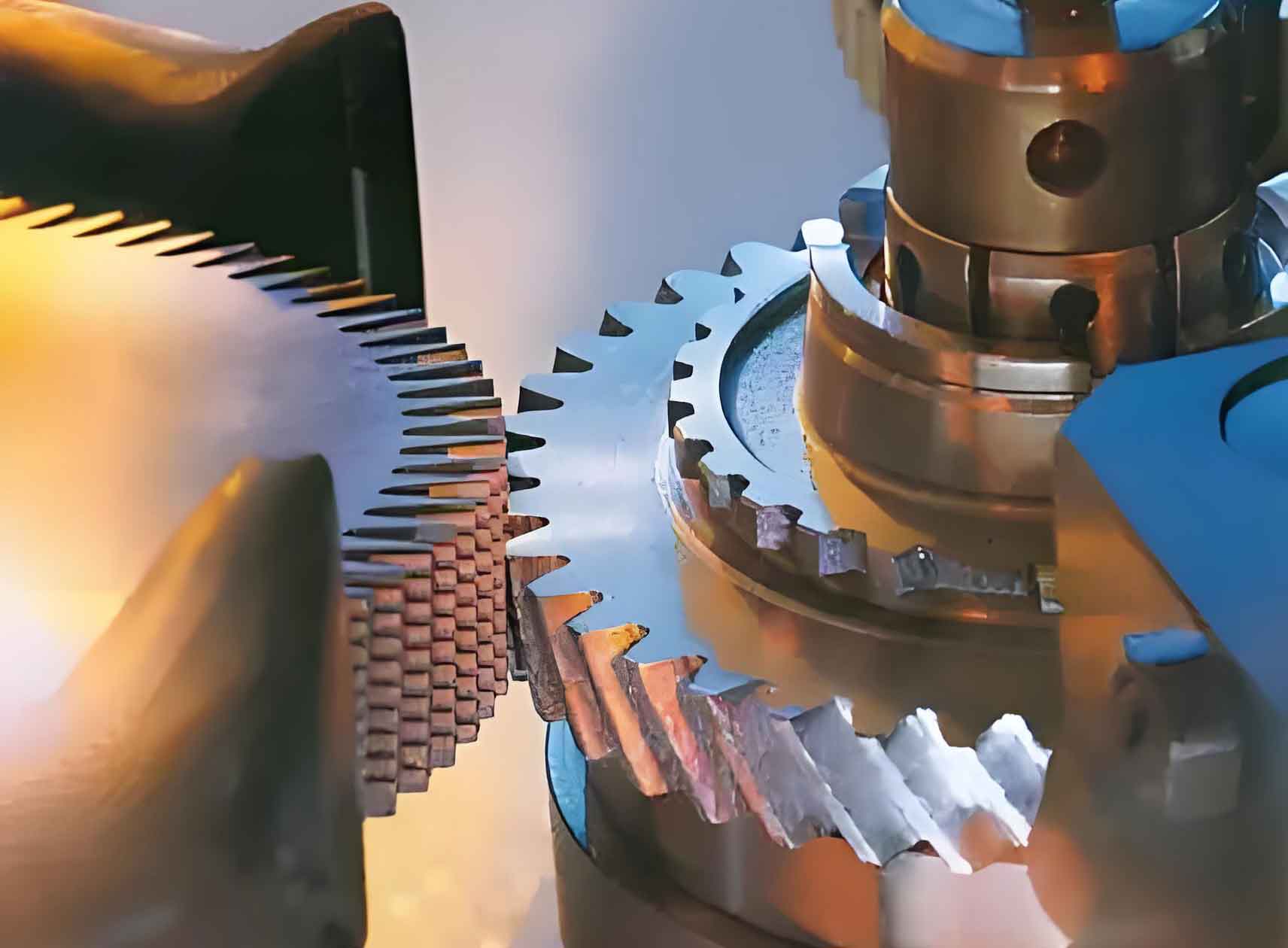
To build a comprehensive prediction model for gear shaving tooth profile concave error, the first step is to establish a detailed analytical model of the gear shaving process that incorporates installation errors. The primary installation errors considered are the axis crossing angle error $\Delta\Sigma$, the center distance error $\Delta a$, and the synchronization errors of the two high-speed axes, $\Delta\omega_1$ for the cutter and $\Delta\omega_2$ for the workpiece. These errors directly affect the relative position and motion between the cutter and workpiece, thereby altering the meshing conditions and ultimately reflecting on the tooth profile error. The geometric model for gear shaving with these installation errors is defined in a coordinate system where the cutter and workpiece axes are crossed. The modified parameters due to errors are:
$$ \Sigma’ = \Sigma + \Delta\Sigma $$
$$ a’ = a + \Delta a $$
$$ \omega_1′ = \omega_1 + \Delta\omega_1 $$
$$ \omega_2′ = \omega_2 + \Delta\omega_2 $$
Here, $\Sigma$ is the nominal axis crossing angle, $a$ is the nominal center distance, $\omega_1$ is the cutter angular velocity, and $\omega_2$ is the workpiece angular velocity. The relative sliding velocity $\mathbf{V}$ at a meshing point with coordinates $(x, y, z)$ in the fixed coordinate system can be derived from the kinematic relationship:
$$ \begin{cases} V_x = -\omega_2′ z \sin\Sigma’ + \omega_2′ y \cos\Sigma’ – \omega_1′ y \\ V_y = \omega_1′ x – \omega_2′ (x – a’) \cos\Sigma’ – v_{02} \sin\Sigma’ \\ V_z = \omega_2′ (x – a’) \sin\Sigma’ – v_{02} \cos\Sigma’ \end{cases} $$
where $v_{02}$ is the axial feed velocity of the workpiece. The cutting speed $V_1$, which is the component of $\mathbf{V}$ perpendicular to the cutter edge, is crucial for material removal and is given by:
$$ V_1 = \omega_2′ (x – a’) \sin\Sigma’ \cos\beta_2 + \omega_2′ (x – a’) \cos\Sigma’ \sin\beta_1 + v_{02} \sin\Sigma’ \sin\beta_1 – v_{02} \cos\Sigma’ \cos\beta_2 – \omega_1′ x \sin\beta_1 $$
where $\beta_1$ and $\beta_2$ are the helix angles of the cutter and workpiece, respectively.
Installation errors shift the actual meshing point trajectory. Based on gear meshing theory, the modified meshing point trajectory $r_e^{(2)}$ is expressed as:
$$ r_e^{(2)}(u_2, \theta_2; \Sigma’, a’, \omega_1′, \omega_2′) = M_{21} r^{(1)}(u_1, \theta_1) $$
Here, $r^{(1)}$ is the cutter tooth surface equation, $M_{21}$ is the transformation matrix from the cutter coordinate system to the workpiece coordinate system, and $(u, \theta)$ are the surface parameters. From this trajectory, the induced normal curvature $K$ along the cutter tooth direction at the meshing point can be determined. This curvature influences the contact pressure and material removal rate. A simplified expression for $K$, considering the modified geometry, is:
$$ K = \frac{\sin\lambda – \left[1 – \frac{1}{r_{b1}^2 + P^2} r_{b1} \sin\Sigma’ \cos\Delta_1 + P \cos\Sigma’\right]}{\sqrt{x^2 + y^2 + z^2}} $$
with $\Delta_1 = \arctan\left(\frac{x}{y}\right) – \arcsin\left[r_{b1}(x^2 + y^2)^{-\frac{1}{2}}\right]$, where $r_{b1}$ is the base radius of the cutter, $\lambda$ is a profile rotation parameter, and $P$ is the helical parameter of the cutter surface.
Another critical factor is the depth of cut $a_p$ at the meshing point. In gear shaving, this is not constant but depends on the radial feed, local indentation, and tooth bending. It can be expressed as:
$$ a_p = \Delta f_r + \delta_c + \delta_w $$
where $\Delta f_r$ is the single radial feed increment, $\delta_c$ is the indentation depth due to contact deformation, and $\delta_w$ is the bending deflection of the workpiece tooth. The radial feed increment is related to the total shaving allowance $\Delta$: $\Delta f_r = \frac{\Delta}{2\sin\alpha}$, with $\alpha$ being the normal pressure angle. The indentation $\delta_c$, based on Hertzian contact theory, is: $\delta_c = e \left( \frac{3\pi\lambda F_{nc}}{2 \sum_{i=1}^m K c_i^{3/2}} \right)^{\frac{2}{3}}$, where $e$ is a ratio related to cutter chip flute geometry, $c_i$ depends on principal curvatures, and $F_{nc}$ is the normal cutting force component. The bending deflection $\delta_w$ is modeled by simplifying the gear tooth as a cantilever beam with variable cross-section. For a meshing point A, considering forces from both flanks, $\delta_w = \delta_{F_{AA}w} – \delta_{F_{BA}w}$, where $\delta_{F_{AA}w}$ and $\delta_{F_{BA}w}$ are deflections due to radial force components at A and the opposite flank B, respectively.
Furthermore, center distance error $\Delta a$ directly alters the effective depth of cut. The resulting error in depth of cut $\Delta a_p$ is derived from geometric relations:
$$ \Delta a_p = \sqrt{(z \sin\Sigma’ – y \cos\Sigma’)^2 + (x + a’)^2} \sin\Sigma’ $$
Thus, the comprehensive expression for the depth of cut during each radial feed in gear shaving becomes:
$$ a_p = \frac{\Delta}{2\sin\alpha} + e \left( \frac{3\pi\lambda F_{nc}}{2 \sum_{i=1}^m K c_i^{3/2}} \right)^{\frac{2}{3}} + \sum_{i=1}^n (\delta_{F_{AA}v_i} – \delta_{F_{BA}v_i}) + \sqrt{(z \sin\Sigma’ – y \cos\Sigma’)^2 + (x + a’)^2} \sin\Sigma’ $$
This analytical model integrates installation errors, kinematics, and deformation, providing a foundation for multi-factor coupling in gear shaving analysis.
The core innovation of this approach is the introduction of the mesh point single cutting area $U$ as a coupling parameter. In gear shaving, each mesh point experiences a discrete cutting event per workpiece revolution. The single cutting area represents the cross-sectional area of material removed from the workpiece tooth flank during one such event at a specific meshing point. It effectively encapsulates the combined influence of installation errors, contact ratio, cutting speed, depth of cut, and induced curvature. To derive $U$, consider the single cutting model at a meshing point A. The cutter edge engages the workpiece over a small arc as the gears rotate. Let $\phi_1$, $\phi_2$, and $\phi_3$ be the cutter rotation angles at the start of contact, maximum depth of cut, and end of contact, respectively. The actual local depth of cut $a_p'(\phi)$ varies during this engagement due to the curved contact path and is related to the nominal depth of cut $a_p$ and the induced curvature $K$ along the cutting path $s(\phi)$:
$$ a_p'(\phi) = \begin{cases} a_p(\phi) – \int_{s(\phi)}^{s(\phi_2)} K(\phi) \, ds, & \phi_1 < \phi < \phi_2 \\ a_p(\phi) – \int_{s(\phi_2)}^{s(\phi)} K(\phi) \, ds, & \phi_2 < \phi < \phi_3 \end{cases} $$
where $s(\phi) = \frac{r_{b1} \phi}{2\pi^2} \times 64800$ approximates the arc length along the cutter edge. The cutting length $l$ during this single event is the integral of the cutting speed $V_1$ over the engagement angle: $l = \int V_1(\phi) \, d\phi$. Therefore, the single cutting area $U$ is the integral of the product of the actual depth of cut and the cutting speed:
$$ U = \int_{\phi_1}^{\phi_3} a_p'(\phi) V_1(\phi) \, d\phi $$
This parameter $U$ serves as a powerful synthetic indicator. A larger $U$ at a given meshing point implies more material removal in one stroke, which is hypothesized to correlate strongly with the generation of tooth profile concave error in gear shaving.
To establish a quantitative prediction model for the gear shaving tooth profile concave error $E$ (typically measured as the profile form deviation in millimeters) and its center location $\theta$ (the profile roll angle where the concavity is deepest), I utilize a machine learning approach. The maximum single cutting area $U_{\text{max}}$ and minimum single cutting area $U_{\text{min}}$ along the tooth profile, along with the profile roll angle $\theta_{\text{max}}$ corresponding to $U_{\text{max}}$, are selected as input features. These features capture the extreme conditions of material removal. The output targets are the error magnitude $E$ and its center $\theta$. For the predictive modeling, a backpropagation (BP) neural network is employed but enhanced with a genetic algorithm (GA) for optimization—hence a GA-BP network. The GA optimizes the initial weights and thresholds of the BP network, overcoming local minima and improving prediction accuracy. The fitness function for the GA is the inverse of the mean squared error (MSE):
$$ f(x) = \frac{1}{\frac{\sum (T – O)^2}{N}} $$
where $T$ is the target output, $O$ is the network output, and $N$ is the number of samples. The network architecture includes an input layer with three neurons ($U_{\text{max}}$, $U_{\text{min}}$, $\theta_{\text{max}}$), a hidden layer with 10 neurons, and an output layer with two neurons ($E$, $\theta$). The training parameters are set with a learning rate of 0.01, a target error of 0.0001, and up to 10,000 epochs.
For experimental validation, a series of gear shaving tests were conducted. The workpiece gear is a small-module gear with 17 teeth, module 4.2333, pressure angle 20°, and addendum modification coefficient 0.0468. Four different shaving cutters were selected, varying in number of teeth, helix angle, and addendum modification to achieve different contact ratios, as summarized in the table below.
| Parameter | Cutter 1 | Cutter 2 | Cutter 3 | Cutter 4 |
|---|---|---|---|---|
| Number of Teeth | 53 | 52 | 53 | 52 |
| Module | 4.2333 | 4.2333 | 4.2333 | 4.2333 |
| Pressure Angle (°) | 20 | 20 | 20 | 20 |
| Helix Angle (°) | 15 | 15 | 10 | 10 |
| Addendum Modification Coef. | -0.3793 | -0.3744 | -0.3649 | -0.3603 |
| Contact Ratio | 1.8294 | 1.7712 | 1.7133 | 1.6548 |
The gear shaving process parameters were varied within practical ranges: spindle speed $n$ (6, 8, 10, 12 r/s), radial feed rate $V_{\text{rad}}$ (3.3, 3.9, 4.5, 5.8 µm/s), and axial feed rate $V_{\text{ax}}$ (0.5, 0.6, 0.85, 1.0 mm/s). Installation errors were simulated by deliberately introducing small adjustments on the machine tool: axis crossing angle error $\Delta\Sigma$ (0.1° to 0.7°), center distance error $\Delta a$ (0.01 to 0.06 mm), and synchronization errors $\Delta\omega_1$, $\Delta\omega_2$ (0.01 to 0.05 r/min). For each parameter combination, the workpiece gear was shaved on a YW423 gear shaving machine, and the resulting tooth profile was measured using a GM3040a universal gear measuring instrument to obtain the actual concave error $E$ and its center position $\theta$. Simultaneously, the corresponding single cutting area parameters were calculated using the derived analytical models for each test condition.
A total of 24 parameter sets were tested. Following the principle of a single variable, 14 sets of data from the right tooth flanks were used to train the GA-BP prediction model, and the remaining 10 sets were used for validation. The calculated single cutting area extremes and the model predictions are compared with measured values in the following table.
| Data No. | $U_{\text{max}}$ (µm²) | $U_{\text{min}}$ (µm²) | $\theta_{\text{max}}$ (°) | Predicted $E$ (mm) | Measured $E$ (mm) | Error in $E$ (%) | Predicted $\theta$ (°) | Measured $\theta$ (°) | Error in $\theta$ (%) |
|---|---|---|---|---|---|---|---|---|---|
| 1 | 2.157 | 0.745 | 27.11 | 0.0303 | 0.0321 | 5.56 | 27.57 | 26.96 | 2.26 |
| 2 | 2.349 | 0.846 | 28.57 | 0.0249 | 0.0267 | 6.48 | 29.08 | 27.99 | 3.89 |
| 3 | 2.235 | 0.694 | 27.76 | 0.0297 | 0.0319 | 6.78 | 28.99 | 27.95 | 3.72 |
| 4 | 2.219 | 0.679 | 27.78 | 0.0315 | 0.0330 | 4.53 | 28.47 | 27.20 | 4.67 |
| 5 | 1.216 | 0.397 | 25.45 | 0.0213 | 0.0229 | 6.95 | 25.37 | 25.76 | 1.51 |
| 6 | 1.516 | 0.541 | 26.24 | 0.0231 | 0.0249 | 7.15 | 26.66 | 26.53 | 0.49 |
| 7 | 1.624 | 0.467 | 26.78 | 0.0239 | 0.0261 | 8.34 | 27.48 | 26.71 | 2.88 |
| 8 | 1.245 | 0.347 | 25.54 | 0.0227 | 0.0246 | 7.76 | 26.42 | 26.38 | 0.15 |
| 9 | 0.804 | 0.216 | 24.78 | 0.0181 | 0.0194 | 6.46 | 25.23 | 25.45 | 0.86 |
| 10 | 0.756 | 0.214 | 24.54 | 0.0160 | 0.0176 | 9.35 | 24.92 | 25.28 | 1.42 |
The results demonstrate the effectiveness of the multi-source coupled prediction model for gear shaving. The average prediction error for the concave error magnitude $E$ is 6.93%, with a maximum error of 9.35% (or 2.2 µm). For the center position $\theta$, the average error is 2.19%, with a maximum of 4.67% (or 1.09°). These low error levels confirm that the model, based on the single cutting area parameter, can accurately predict both the size and location of the tooth profile concave error in gear shaving. This validates the premise that coupling multiple factors into the single cutting area is a viable strategy for quantitative prediction.
Having established the predictive model, I now delve into analyzing the influence of the single cutting area on the gear shaving tooth profile concave error. The relationship between $U$ and $E$ is not linear. As observed from the data and further analysis, the concave error initially increases with the single cutting area but begins to decrease after $U$ exceeds a certain threshold. This can be explained by the self-correcting nature of the gear shaving process. Gear shaving involves multiple passes and repeated cuts. If an initial cut removes an excessive amount of material at a specific point (high $U$), it creates a local concavity. However, this concavity alters the local geometry, reducing the induced normal curvature and consequently the effective depth of cut in subsequent passes at that same point. Therefore, the single cutting area for that location in later passes decreases. If the initial $U$ is very large, this corrective reduction happens more rapidly, leading to a net reduction in the final profile deviation. Thus, there exists an optimal range of $U$ where the concave error is maximized; outside this range, error mitigation occurs. This insight is crucial for process optimization in gear shaving: one should avoid parameter combinations that yield single cutting areas near this peak region.
Furthermore, the center of the concave error $\theta$ closely aligns with the position of the maximum single cutting area $U_{\text{max}}$ along the tooth profile. As $U$ increases overall, the location of $U_{\text{max}}$ tends to shift toward the tooth tip, and consequently, the error center $\theta$ also moves tip-ward. This shift is attributed to the changing force distribution and tooth bending. When radial cutting forces increase, the bending deflection near the tooth tip grows more significantly than near the root due to the cantilever effect. This alters the effective contact and material removal distribution, pushing the point of most severe cutting toward the tip. The strong correlation confirms that the maximum single cutting area is the primary driver determining where the concavity forms during gear shaving.
To provide practical guidance for controlling gear shaving tooth profile concave error, it is essential to understand how various process parameters affect the single cutting area $U$. The table below summarizes the calculated maximum single cutting area $U_{\text{max}}$ for different parameter settings, highlighting the effect of each factor when others are held constant.
| Set No. | Contact Ratio | $V_{\text{ax}}$ (mm/s) | $V_{\text{rad}}$ (µm/s) | $n$ (r/s) | $\Delta\Sigma$ (°) | $\Delta a$ (mm) | $\Delta\omega_1$ (r/min) | $U_{\text{max}}$ (µm²) |
|---|---|---|---|---|---|---|---|---|
| 1 | 1.8294 | 1.0 | 5.8 | 6 | 0.1 | 0.01 | 0.01 | 2.157 |
| 2 | 1.7712 | 1.0 | 5.8 | 6 | 0.1 | 0.01 | 0.01 | 2.349 |
| 3 | 1.7133 | 1.0 | 5.8 | 6 | 0.1 | 0.01 | 0.01 | 2.235 |
| 4 | 1.6548 | 1.0 | 5.8 | 6 | 0.1 | 0.01 | 0.01 | 2.219 |
| 5 | 1.8294 | 1.0 | 5.8 | 6 | 0.1 | 0.01 | 0.01 | 1.216 |
| 6 | 1.8294 | 1.0 | 5.8 | 8 | 0.1 | 0.01 | 0.01 | 1.516 |
| 7 | 1.8294 | 0.5 | 5.8 | 6 | 0.1 | 0.01 | 0.01 | 1.624 |
| 8 | 1.8294 | 0.85 | 5.8 | 6 | 0.1 | 0.01 | 0.01 | 1.245 |
| 9 | 1.8294 | 1.0 | 3.3 | 6 | 0.1 | 0.01 | 0.01 | 0.804 |
| 10 | 1.8294 | 1.0 | 5.8 | 6 | 0.3 | 0.01 | 0.01 | 1.956 |
| 11 | 1.8294 | 1.0 | 5.8 | 6 | 0.1 | 0.03 | 0.01 | 1.534 |
| 12 | 1.8294 | 1.0 | 5.8 | 6 | 0.1 | 0.01 | 0.03 | 1.227 |
From this analysis, several key trends for gear shaving process control emerge:
- Contact Ratio: The effect of contact ratio on single cutting area is non-monotonic. As the contact ratio increases from 1.6548 to 1.7712, $U_{\text{max}}$ initially decreases, but then increases as the ratio further rises to 1.8294. This is because a higher contact ratio reduces the induced normal curvature (which tends to decrease cutting area) but increases the effective cutting length (which tends to increase it). Beyond a certain point, the length effect dominates. Therefore, simply maximizing contact ratio is not always beneficial for minimizing concave error in gear shaving; an optimal range exists.
- Feed Rates and Speed: The radial feed rate $V_{\text{rad}}$ and axial feed rate $V_{\text{ax}}$ are positively correlated with $U_{\text{max}}$. Higher feeds directly increase the depth of cut and cutting speed, respectively, leading to a larger single cutting area. Conversely, the spindle speed $n$ is negatively correlated with $U_{\text{max}}$. A higher spindle speed increases the relative sliding velocity, which, for a given depth, can reduce the effective engagement time per cut, thus decreasing the cutting area. Therefore, to control concave error in gear shaving, one can consider reducing feed rates and increasing spindle speed, within practical limits.
- Installation Errors: Axis crossing angle error $\Delta\Sigma$ and center distance error $\Delta a$ both show a strong positive correlation with $U_{\text{max}}$. These errors directly introduce geometric deviations that increase the effective depth of cut, significantly amplifying the single cutting area. In contrast, the high-speed axis synchronization errors $\Delta\omega_1$ and $\Delta\omega_2$ have a relatively minor impact. This underscores the critical importance of precise machine setup and alignment in gear shaving to minimize installation errors, particularly axis angle and center distance, for controlling tooth profile quality.
The overarching conclusion is that the single cutting area $U$ serves as a comprehensive indicator of the multi-source coupling in gear shaving. By monitoring and controlling parameters to keep $U$ within a moderate range—avoiding the peak region—manufacturers can effectively suppress the formation of tooth profile concave error.
In summary, this work has developed and validated a multi-source coupled prediction model for gear shaving tooth profile concave error. The model integrates installation errors, kinematic parameters, and gear geometry into a unified analytical framework, culminating in the concept of the mesh point single cutting area. This parameter encapsulates the combined effect of multiple factors influencing the gear shaving process. Using a GA-BP neural network, the model successfully predicts both the magnitude and location of the concave error with high accuracy, as confirmed by experimental tests. The analysis reveals that excessive single cutting area is the primary cause of concave error formation in gear shaving, but a self-correcting mechanism exists at very high removal rates. Furthermore, the error center is dictated by the location of maximum single cutting area. Practical insights for process optimization include selecting an appropriate contact ratio, reducing feed rates, increasing spindle speed, and most importantly, minimizing axis crossing angle and center distance errors during machine setup. This research advances the understanding of gear shaving mechanics beyond single-factor analyses, providing a robust tool for predicting and controlling tooth profile errors, thereby contributing to the manufacture of higher precision gears with improved performance and longevity. Future work could extend this coupling approach to other gear finishing processes or incorporate dynamic effects and thermal influences for an even more comprehensive model.