
In the realm of gear manufacturing, gear shaving stands out as a pivotal finishing process that enhances the precision and surface integrity of involute cylindrical gears. Among its variants, radial gear shaving has emerged as a superior technique, offering notable advantages over conventional axial gear shaving. As a researcher delving into this field, I have explored the underlying principles and practical challenges associated with radial gear shaving cutters. This article presents my comprehensive analysis, focusing on the tooth surface formation, computational methods, and grinding solutions for radial gear shaving cutters. The goal is to facilitate the manufacturing and regrinding of these cutters, thereby promoting the widespread adoption of radial gear shaving in industrial applications. Throughout this discussion, the term gear shaving will be frequently emphasized to underscore its centrality in this context.
Radial gear shaving distinguishes itself by enabling continuous line contact between the cutter and workpiece tooth surfaces during the shaving process. This contrasts with conventional gear shaving, where point contact often leads to uneven wear and mid-concavity defects. The radial gear shaving method not only boosts efficiency but also ensures uniform cutting force distribution, making it ideal for precision finishing of multi-stage gears.
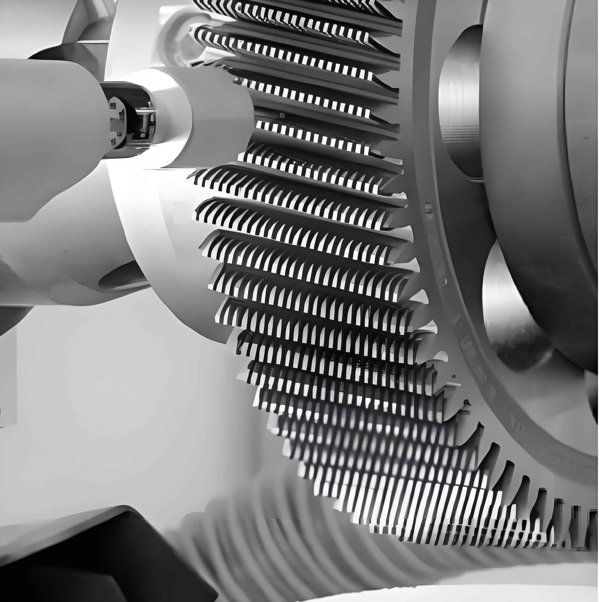
The image above illustrates the typical setup for gear shaving, highlighting the interaction between the cutter and gear. However, the complex tooth surface geometry of radial gear shaving cutters poses significant manufacturing hurdles, as it deviates from standard involute profiles. To address this, I have conducted detailed investigations into the theoretical tooth surface, followed by fitting strategies using conical grinding wheels. This work aims to bridge the gap between theory and practice, ensuring that radial gear shaving can be reliably implemented.
The foundation of radial gear shaving lies in spatial meshing theory. Consider a coordinate system where the workpiece gear (denoted as gear 1) has its axis aligned with the z-axis, and the radial gear shaving cutter (gear 2) has its axis aligned with the z’-axis. The angle between these axes is denoted as Σ, representing the crossed-axis configuration. The fundamental meshing condition requires that at any contact point, the common normal vector is perpendicular to the relative velocity vector. This can be expressed through the meshing equation:
$$ \mathbf{n} \cdot \mathbf{v}^{(12)} = 0 $$
Here, \(\mathbf{n}\) is the normal vector to the tooth surface, and \(\mathbf{v}^{(12)}\) is the relative velocity between the two gears. To derive explicit equations, let \(\omega^{(1)}\) and \(\omega^{(2)}\) be the angular velocity vectors of the workpiece and cutter, respectively. In the fixed coordinate system, these can be written as:
$$ \omega^{(1)} = \omega_1 \begin{bmatrix} 0 \\ 0 \\ 1 \end{bmatrix}, \quad \omega^{(2)} = \omega_2 \begin{bmatrix} \sin\Sigma \\ 0 \\ \cos\Sigma \end{bmatrix} $$
The relative velocity at a point \(\mathbf{r}\) on the tooth surface is given by:
$$ \mathbf{v}^{(12)} = \omega^{(1)} \times \mathbf{r} – \omega^{(2)} \times (\mathbf{r} – \mathbf{a}) $$
where \(\mathbf{a}\) is the vector connecting the two axes origins, with magnitude \(a\) representing the center distance. For a helical involute gear as the workpiece, the tooth surface parametric equations in its local coordinate system are:
$$ \begin{cases}
x_1 = r_b [\cos(u + \theta_0) + u \sin(u + \theta_0)] \\
y_1 = r_b [\sin(u + \theta_0) – u \cos(u + \theta_0)] \\
z_1 = p \cdot v
\end{cases} $$
In these equations, \(r_b\) is the base radius, \(u\) is the involute roll angle, \(\theta_0\) is the starting angle of the involute, \(p\) is the spiral parameter defined as \(p = r_b \tan\beta_b\) (with \(\beta_b\) being the base helix angle), and \(v\) is a helical parameter. The normal vector components are derived through partial derivatives:
$$ \mathbf{n}_1 = \begin{bmatrix}
-\frac{\partial z_1}{\partial v} \frac{\partial y_1}{\partial u} + \frac{\partial y_1}{\partial v} \frac{\partial z_1}{\partial u} \\
-\frac{\partial x_1}{\partial v} \frac{\partial z_1}{\partial u} + \frac{\partial z_1}{\partial v} \frac{\partial x_1}{\partial u} \\
-\frac{\partial y_1}{\partial u} \frac{\partial x_1}{\partial v} + \frac{\partial x_1}{\partial u} \frac{\partial y_1}{\partial v}
\end{bmatrix} $$
Substituting the parametric expressions yields:
$$ \mathbf{n}_1 = \begin{bmatrix}
p \sin(u + \theta_0) \\
-p \cos(u + \theta_0) \\
r_b u
\end{bmatrix} $$
Transforming these into the fixed coordinate system and applying the meshing condition leads to the meshing equation specific to radial gear shaving:
$$ \omega_1 [y \cos\Sigma – (z – a) \sin\Sigma] n_x + \omega_1 [ -x \cos\Sigma ] n_y + \omega_1 [x \sin\Sigma] n_z – \omega_2 [ -y n_x + x n_y ] = 0 $$
After algebraic manipulation, for a helical workpiece gear, the meshing equation simplifies to:
$$ \omega_1 r_b u \cos\Sigma – \omega_1 p \sin\Sigma \cos(u + \theta_0) + \omega_2 [p \cos(u + \theta_0) – r_b u \sin\Sigma] = 0 $$
This equation relates the parameters \(u\), \(v\), and the rotation angle \(\phi\) of the cutter. Solving it simultaneously with the tooth surface equations transformed into the cutter coordinate system yields the theoretical tooth surface of the radial gear shaving cutter. The transformation from workpiece coordinates \((x_1, y_1, z_1)\) to cutter coordinates \((x_2, y_2, z_2)\) involves rotation and translation:
$$ \begin{bmatrix}
x_2 \\
y_2 \\
z_2
\end{bmatrix} = \begin{bmatrix}
\cos\phi & \sin\phi & 0 \\
-\sin\phi & \cos\phi & 0 \\
0 & 0 & 1
\end{bmatrix} \begin{bmatrix}
x_1 \\
y_1 \\
z_1 – a
\end{bmatrix} $$
By discretizing the parameters, I computed cross-sectional profiles of the cutter tooth surface. Each profile was then fitted with an involute curve to assess deviations. The results, summarized in Table 1, show that the base radius varies slightly along the tooth length, but the normal errors are minimal, on the order of micrometers. This confirms that the tooth surface is nearly involute but twisted, necessitating advanced grinding approaches.
| Cross-Section Position \(z\) (mm) | Fitted Involute Base Radius \(r_{b,fit}\) (mm) | Maximum Normal Error \(\Delta\) (μm) |
|---|---|---|
| -10 | 100.123 | 0.05 |
| -5 | 100.125 | 0.06 |
| 0 | 100.128 | 0.04 |
| 5 | 100.130 | 0.07 |
| 10 | 100.132 | 0.05 |
The twisted nature of the tooth surface implies that conventional grinding with a plane wheel would introduce significant errors. Therefore, I turned to a fitting strategy using a conical grinding wheel, which better approximates the complex geometry. This involves two main steps: first, calculating the imaginary rack tooth surface that is conjugate to the cutter tooth surface; second, optimizing the conical wheel parameters to fit this rack surface. The concept of an imaginary rack arises from the gear-rack meshing principle commonly employed in gear grinding machines like the Y7125 model.
To derive the imaginary rack tooth surface, consider the coordinate system where the cutter rotates about its axis, and the rack translates along a direction perpendicular to the cutter axis. The meshing condition here is based on the theorem that the normal at any contact point must pass through the pitch point. For a given point on the cutter tooth surface with coordinates \((x_2, y_2, z_2)\), the condition for it to be in contact with the rack is expressed through the angle \(\phi\) of cutter rotation:
$$ \tan\phi = \frac{y_2 – y_p}{x_2 – x_p} $$
Here, \((x_p, y_p)\) are the coordinates of the pitch point, which for a standard gear-rack pair is at a distance \(r_p\) (pitch radius) from the cutter center. Using the normal vector components \(n_{x2}\) and \(n_{y2}\) from the cutter tooth surface, the relationship simplifies to:
$$ \phi = \arctan\left( \frac{n_{y2}}{n_{x2}} \right) + \frac{\pi}{2} $$
The rack tooth surface coordinates \((x_r, y_r, z_r)\) in the rack coordinate system are then obtained through transformation:
$$ \begin{cases}
x_r = x_2 \cos\phi + y_2 \sin\phi – r_p \phi \\
y_r = -x_2 \sin\phi + y_2 \cos\phi + r_p \\
z_r = z_2
\end{cases} $$
This yields a set of points representing the rack tooth surface. Due to the cutter’s twisted tooth surface, the rack surface is also non-standard, requiring approximation with a simple geometry for grinding purposes. I propose using a conical wheel, as its surface can be described by a few parameters and offers flexibility in matching curved profiles.
The conical wheel surface equation in its local coordinate system \((X_w, Y_w, Z_w)\) is given by:
$$ \begin{cases}
X_w = R – s \sin\beta \\
Y_w = s \cos\beta \cos\gamma \\
Z_w = s \cos\beta \sin\gamma + Z_0
\end{cases} $$
where \(R\) is the wheel radius (at the largest diameter), \(\beta\) is the cone half-angle, \(\gamma\) is the tilt angle relative to the rack coordinate system, \(Z_0\) is an axial offset, and \(s\) is a parameter along the cone generator. To fit this to the rack tooth surface, both are transformed into a common coordinate system, denoted as \((X’, Y’, Z’)\), which aligns with the rack’s pitch plane. The transformation involves rotations and translations based on the machine setup angles.
For a given cross-section of the rack at position \(Z’ = Z_c\), the intersection of the conical surface with this plane yields a curve. The theoretical rack points in that section have coordinates \((X’_{r,i}, Y’_{r,i}, Z_c)\). The error between the conical curve and these points is approximated by the difference in the \(Y’\) coordinate, as the rack profile is primarily aligned with the \(X’\)-axis. Thus, the normal error for point \(i\) is:
$$ \Delta_i = Y’_{r,i} – Y’_{w,i} $$
where \(Y’_{w,i}\) is the \(Y’\) coordinate on the conical curve corresponding to \(X’_{r,i}\). The objective is to minimize the sum of squared errors over all points across multiple cross-sections. The optimization problem is formulated as:
$$ \text{Minimize } F(R, \beta, \gamma, Z_0) = \sum_{j=1}^{m} \sum_{i=1}^{n_j} \left( Y’_{r,i,j} – Y’_{w,i,j} \right)^2 $$
Here, \(j\) indexes the cross-sections, and \(n_j\) is the number of points in section \(j\). Constraints are applied based on practical grinding limits, such as wheel size and angle ranges. I developed a numerical optimization program using gradient-based methods to solve this problem. The algorithm iteratively adjusts the parameters to converge to an optimal set.
To validate the approach, I applied it to a typical radial gear shaving cutter scenario. The workpiece gear parameters were: module \(m_n = 3 \, \text{mm}\), number of teeth \(z_1 = 30\), helix angle \(\beta_1 = 15^\circ\) (right-hand), pressure angle \(\alpha_n = 20^\circ\), and face width 20 mm. The cutter parameters were: number of teeth \(z_2 = 80\), interaxial angle \(\Sigma = 15^\circ\). The computed optimal conical wheel parameters and resulting errors are listed in Table 2.
| Parameter | Optimal Value | Units |
|---|---|---|
| Wheel Radius \(R\) | 150.25 | mm |
| Cone Half-Angle \(\beta\) | 2.85 | degrees |
| Tilt Angle \(\gamma\) | 1.20 | degrees |
| Axial Offset \(Z_0\) | -0.05 | mm |
| Maximum Normal Error | 0.008 | mm |
| Average Error | 0.002 | mm |
The results demonstrate that the conical wheel can accurately approximate the imaginary rack tooth surface, with maximum errors well below 0.01 mm, which is acceptable for precision gear shaving cutters. This indicates that the grinding process on machines like the Y7125 can be effectively adapted for radial gear shaving cutters by setting the wheel parameters as per the optimization output.
Further analysis involved sensitivity studies to understand how parameter variations affect the gear shaving quality. For instance, Table 3 shows the impact of small changes in the cone angle \(\beta\) on the fitting error, holding other parameters constant at their optimal values.
| \(\beta\) Deviation (degrees) | Maximum Error Increase (mm) | Comment |
|---|---|---|
| -0.5 | 0.005 | Acceptable |
| -0.2 | 0.002 | Negligible |
| 0 (optimal) | 0.000 | Baseline |
| +0.2 | 0.002 | Negligible |
| +0.5 | 0.006 | Acceptable |
Such insights are crucial for setting tolerances in practical gear shaving operations. Additionally, the optimization program can be extended to account for dynamic factors like wheel wear and machine vibrations, further refining the gear shaving process.
In conclusion, this research provides a robust methodology for grinding radial gear shaving cutters used in involute cylindrical gear finishing. By deriving the theoretical tooth surface through spatial meshing equations and employing a conical wheel fitting strategy via an imaginary rack, I have addressed key manufacturing challenges. The optimization program ensures that the grinding parameters are tailored to minimize errors, making radial gear shaving more accessible and reliable. As gear shaving continues to evolve, such advancements will enhance efficiency and precision in gear production, solidifying radial gear shaving as a preferred technique in high-quality gear manufacturing. Future work may explore real-time adaptive control during grinding and the application to other gear types, further expanding the horizons of gear shaving technology.