
Gear shaving stands as one of the primary finishing methods for non-hardened cylindrical gears. The process can achieve a gear quality grade up to 6 (per GB/T 10095.1-2008) and a surface roughness (Ra) of 0.8 to 0.2 μm. Its high productivity, operational convenience, and long tool life have led to its widespread adoption in mass production.
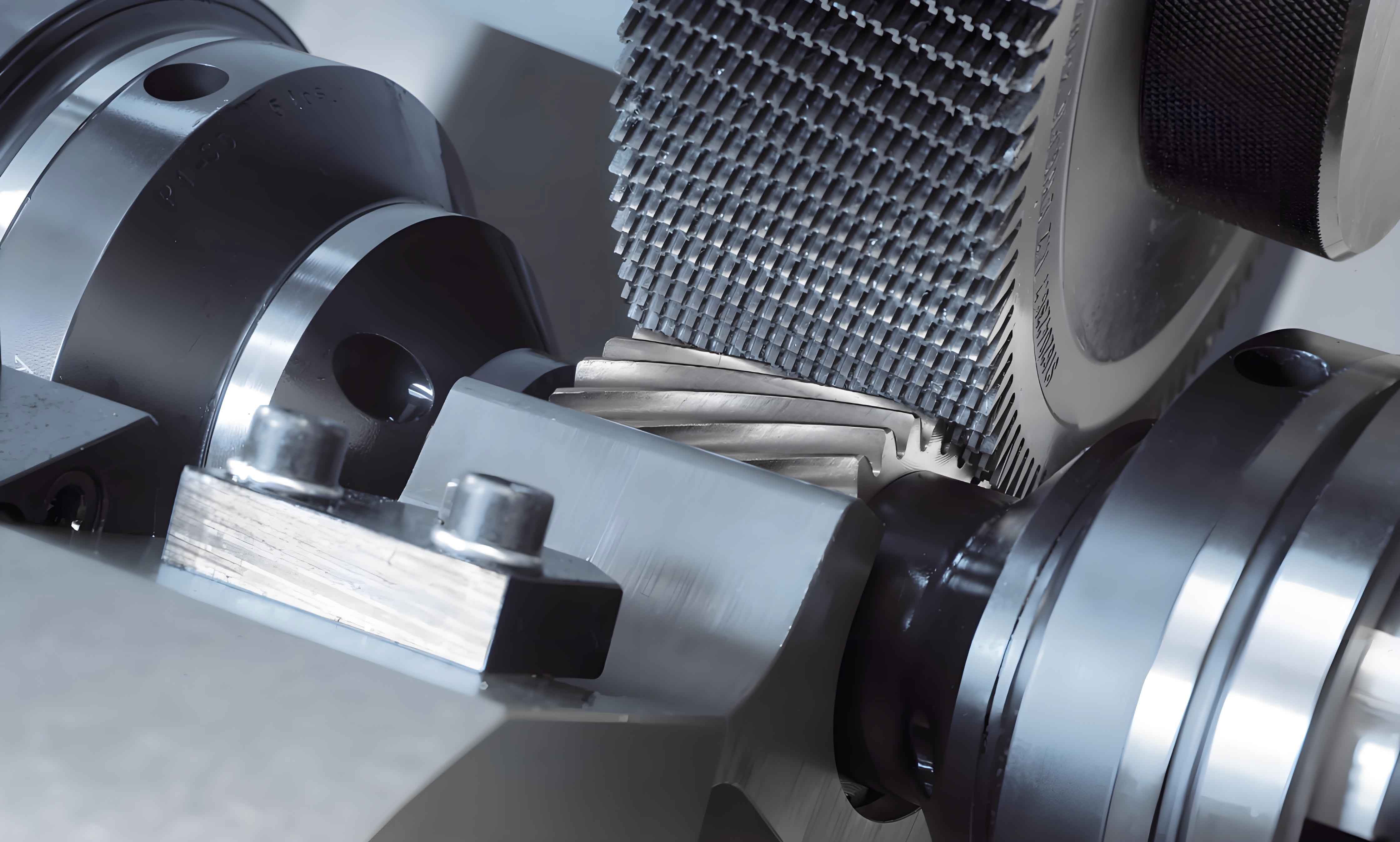
The gear shaving process utilizes a cutter that essentially resembles a gear, with numerous small grooves cut into its tooth flanks to form cutting edges. The cutter and the workpiece gear are mounted on crossed axes, engaging as a pair of helical gears. The shaft angle Σ is determined by the helix angles of the workpiece gear (β_g) and the shaving cutter (β_c):
$$ \Sigma = \beta_g \pm \beta_c $$
The plus sign is used when the helix directions are the same, and the minus sign when they are opposite. The cutter, driven by the machine spindle, rotates and drives the workpiece gear. The relative sliding motion between the meshing tooth surfaces performs the cutting action. A reciprocating traverse motion is applied to cover the entire face width, and a radial infeed is used to reach the required depth. To ensure equal material removal from both flanks of the gear, the rotation direction of the gear shaving cutter is periodically reversed.
Phenomenon of Mid-Profile Concavity and Conventional Solutions
The gear shaving process is inherently complex, involving simultaneous cutting, plowing, and sliding actions. Cutting angles and forces vary continuously during the engagement, and the drive between the cutter and gear is unconstrained. Consequently, gears shaved with a standard involute shaving cutter do not possess a perfect involute profile. A common defect, especially when shaving spur gears with a standard disk-type cutter, is a concavity in the tooth profile near the pitch point. This is widely known as the “mid-profile concavity” or “shaving dip” phenomenon.
The effective solution to this problem is to modify or “dress” the profile of the gear shaving cutter. Two conventional methods are prevalent:
- Template-Based Dressing: The concavity curve of the shaved gear is first measured. A template is then manufactured based on this curve. On a dedicated sharpening machine, a diamond dressing tool shapes the grinding wheel according to this template. The dressed wheel is then used to re-grind the shaving cutter.
- CNC-Controlled Dressing: This method replaces the physical template with a computer program. On a specialized grinder, a CNC system controls the path of a diamond dresser to impart the required form onto the grinding wheel, which subsequently dresses the gear shaving cutter.
Both methods share significant drawbacks: they require dedicated, expensive equipment and specialized technical expertise; the dressing data (template or program) must be recalculated for different gear parameters and for new vs. worn cutters, making the process complex; and several trial shaving and re-dressing iterations are often needed. Therefore, the industry has a pressing need for a simpler, more reliable, and efficient dressing method for gear shaving cutters.
Theoretical Foundation for a Novel Dressing Method
The genesis of the mid-profile concavity error is multifaceted, stemming from a dynamic synthesis of various error sources during the gear shaving process, including machine tool inaccuracies, cutter geometry, and process parameters. Our fundamental hypothesis is to not meticulously control each error factor but to strategically utilize the aggregate effect.
The core idea is to use the “concavity effect” to counteract itself—to eliminate the mid-profile concavity by intentionally imparting a complementary form onto the cutter. This is achieved through a “reverse cutting” or “grinding-in” process. A specially designed dressing wheel, featuring a hard abrasive-laden tooth surface, is mounted in the workpiece position on the gear shaving machine. Its key parameters are derived from the target workpiece gear.
When this dressing wheel engages with the shaving cutter under standard gear shaving motions, the hard abrasive teeth of the dressing wheel act upon the relatively softer cutter teeth. According to the principle of reverse cutting, the systemic error tendencies that normally cause concavity on the workpiece are now transferred to the cutter. Therefore, the gear shaving cutter itself develops a corresponding concavity in its profile. Subsequently, when this pre-dressed cutter is used to shave a standard gear, its intentional profile error compensates for the process-induced error, resulting in a final gear tooth profile that is close to the ideal involute.
Furthermore, because this dressing process occurs under conditions nearly identical to actual gear shaving (same machine, similar kinematics), it inherently compensates for random process-related errors specific to that setup. Hence, we term this approach the “Random Dressing Method.”
Mathematical Modeling of the Compensation Principle
The profile deviation on a shaved gear, Δ_g(ξ), at a roll angle ξ, can be considered a function of the ideal cutter profile C_id(ξ), the actual machine-cutter-workpiece system state S, and process parameters P:
$$ \Delta_g(\xi) = F(C_{id}(\xi), S, P) $$
Typically, F(·) leads to Δ_g(ξ) < 0 (concavity) around the pitch point ξ_p. The goal of dressing is to find a modified cutter profile C_mod(ξ) such that when used under the same S and P, the output deviation is minimized:
$$ \min \left( \Delta_g'(\xi) = F(C_{mod}(\xi), S, P) \right) \approx 0 $$
In the random dressing method, we define a dressing wheel profile D(ξ). The engagement between the initial cutter C_init(ξ) and D(ξ) under a similar functional G (representing the reverse cutting process) produces the modified cutter profile:
$$ C_{mod}(\xi) = G(C_{init}(\xi), D(\xi), S_d, P_d) $$
By designing D(ξ) to induce an error -Δ_g(ξ) onto C_init(ξ) via G(·), we get C_mod(ξ) = C_init(ξ) – k·Δ_g(ξ), where k is a transfer coefficient. Substituting back, the final gear error becomes:
$$ \Delta_g'(\xi) = F(C_{init}(\xi) – k \cdot \Delta_g(\xi), S, P) \approx \Delta_g(\xi) – k’ \cdot \Delta_g(\xi) $$
where k’ is an effective compensation coefficient. With proper calibration (achieved by adjusting dressing parameters P_d), k’ → 1, leading to Δ_g'(ξ) → 0.
Practical Implementation and Process Guidelines
The successful application of the Random Dressing Method hinges on the design of the dressing wheel and the selection of process parameters.
1. Dressing Wheel Design and Fabrication:
The dressing wheel is a critical component. Its base body should have a geometric configuration (module, pressure angle, helix angle, number of teeth) closely matching the workpiece gear to replicate the meshing conditions. The tooth flanks are coated or embedded with hard abrasives, such as diamond or cubic boron nitride (CBN) grains. The bond material can be metallic, resinoid, or vitrified, chosen for its ability to retain grains while allowing slight wear to maintain a sharp cutting surface. The abrasive grit size directly influences the surface finish of the dressed gear shaving cutter; a finer grit is preferred for a smoother cutter surface.
2. Dressing Process Parameters:
The dressing operation is performed on a standard gear shaving machine. The following parameters must be optimized:
- Shaft Angle (Σ_d): Similar to the shaving process, this affects the sliding velocity and cutting action. It is typically set equal to the intended shaving angle Σ.
- Radial Infeed: This controls the depth of material removed from the cutter teeth. It must be carefully controlled to achieve the desired amount of profile modification without over-dressing.
- Reciprocating Stroke and Feed Rate: Ensure the entire face width of the cutter is dressed uniformly.
- Number of Passes and Reversal Cycles: Dressing often requires multiple passes with incremental radial infeeds. The direction of cutter rotation is reversed periodically, just like in actual gear shaving, to dress both flanks evenly.
- Coolant: Amundant coolant is essential to wash away swarf, prevent loading of the dressing wheel, and avoid thermal damage to the cutter.
The table below summarizes a recommended parameter framework for the random dressing process.
| Process Parameter | Description & Consideration | Typical Range/Value |
|---|---|---|
| Dressing Wheel | Base geometry matches workpiece. Abrasive: Diamond/CBN. Grit size: Fine (e.g., 200-400 mesh). | Custom-made per gear spec. |
| Shaft Angle (Σ_d) | Set equal to the production shaving angle. | Σ_d = β_g ± β_c (10°-20° common) |
| Initial Radial Clearance | Gap before infeeding to avoid impact. | 0.1 – 0.2 mm |
| Total Radial Infeed (ΔR) | Main variable controlling modification depth. | 0.02 – 0.08 mm (tuned via trial) |
| Infeed per Pass | Incremental depth per dressing cycle. | 0.005 – 0.015 mm |
| Reciprocating Feed Rate | Speed of axial traverse. | 50 – 150 mm/min |
| Number of Strokes per Pass | Complete traverses per infeed increment. | 4 – 8 |
| Cutter Speed (RPM) | Rotational speed of the shaving cutter. | 80 – 200 RPM |
Results Analysis and Comparative Advantages
Practical implementation of the Random Dressing Method has demonstrated its efficacy. The tooth profile of gears shaved with a randomly dressed cutter shows a significant reduction, and often elimination, of the characteristic mid-profile concavity. The achievable quality consistently meets the 7th grade (with profile form error f_fa greatly reduced), and surface roughness remains within Ra 0.8 to 0.4 μm. Any residual systematic bias or slope in the profile trace can be attributed to minor errors in the basic gear tooth angle. This can be further corrected in a subsequent dressing cycle by slightly adjusting the nominal pressure angle of the dressing wheel.
The advantages of this novel method over traditional approaches are substantial and multifaceted, as summarized in the following comparative table.
| Aspect | Traditional Methods (Template/CNC) | Random Dressing Method |
|---|---|---|
| Underlying Principle | Precise, deterministic correction based on measured error. | Compensation via transfer of systemic & random errors through reverse cutting. |
| Required Equipment | Dedicated, high-precision sharpening/grinding machine with template mechanism or CNC system. | Standard gear shaving machine. Only a custom dressing wheel is needed. |
| Technical Complexity | High. Requires skilled technicians for measurement, template/program design, and machine operation. | Low. Process is similar to standard gear shaving. Operators can be easily trained. |
| Setup & Lead Time | Long. Involves measuring, designing, manufacturing templates/programs, and trial iterations. | Short. Dressing wheel is pre-made. Process setup is quick on the shaving machine. |
| Flexibility & Cost | Low flexibility, high cost per design change. High capital investment for equipment. | High flexibility. New dressing wheel needed for major parameter changes. Very low capital cost. |
| Error Compensation Scope | Primarily compensates for deterministic profile form errors. | Compensates for both deterministic profile errors and random process-specific errors (e.g., machine deflections). |
| Implementation Barrier | High, suitable for large manufacturers. | Low, accessible to small and medium-sized enterprises. |
Conclusion
The Random Dressing Method presents a paradigm shift in addressing the persistent challenge of mid-profile concavity in gear shaving. By leveraging the inherent error generation mechanisms of the gear shaving process itself through a reverse-cutting action with an abrasive dressing wheel, it offers a simple, elegant, and highly effective solution. It eliminates the need for complex, expensive dedicated equipment and reduces reliance on highly specialized labor. The method is characterized by its low cost, operational simplicity, and robust compensation for a range of error sources. This makes it an exceptionally practical and accessible technology for gear manufacturers of all scales seeking to enhance the accuracy and consistency of their gear shaving operations while controlling costs. The successful practice of this method confirms that intelligent utilization of process dynamics can often yield more efficient solutions than attempts at their complete elimination.