
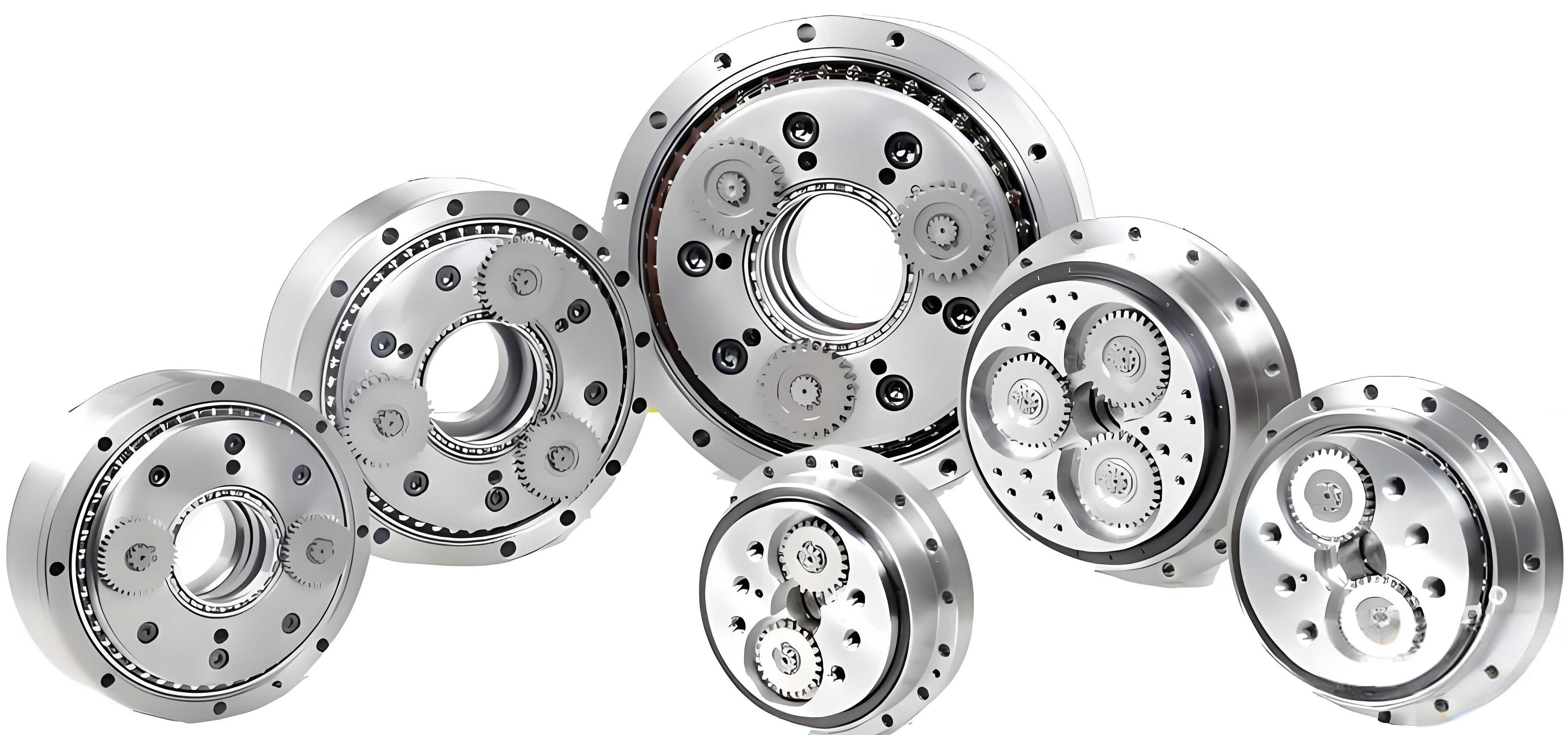
The precision and reliability of core components in high-end manufacturing, such as industrial robots and precision machine tools, are paramount. The rotary vector reducer, a type of precision cycloidal drive, has become the dominant solution for robotic joints due to its exceptional characteristics: compact size, high torsional stiffness, low vibration, wide transmission ratio range, smooth operation, long service life, and high transmission efficiency. However, the design and manufacturing of these reducers are technologically intensive. For a long time, the global market, especially for high-precision applications, has been dominated by a few international companies. Breaking this technological monopoly requires significant advancements in design methodologies, analysis techniques, and verification processes. The core performance metric limiting this progress is transmission error, which directly impacts the positioning accuracy and motion stability of the entire system.
Traditional design approaches for the rotary vector reducer often rely on iterative processes involving allowable stress formulas and safety factor checks. This conventional cycle—”design, verification, prototyping, testing, modification, redesign”—is inherently time-consuming and costly. It presents considerable difficulty in converging on an optimal design solution. While recent research has explored the creation of three-dimensional models and virtual prototype simulations for the rotary vector reducer, significant practical hurdles remain. Manually defining constraints and contacts for the complex assembly within multi-body dynamics simulation software like ADAMS is a tedious and error-prone task. Any modification to the model’s geometric parameters necessitates a complete redefinition of the virtual prototype’s constraints, leading to low efficiency and hindering rapid design exploration. Furthermore, the absence of physical experimental validation often leaves the accuracy of these simulation models in question.
This article presents an integrated methodology that overcomes these challenges by establishing a rapid, automated workflow for building and validating transmission error virtual prototypes of the rotary vector reducer. The core of this method lies in combining parametric three-dimensional modeling with automated constraint definition via macro commands in a dynamics simulation environment, followed by rigorous experimental correlation. The研究对象 is a common model, the RV-40E-81 type rotary vector reducer. This systematic approach significantly reduces the complexity and time associated with virtual prototype creation, providing a practical and efficient tool for the research and development of high-performance rotary vector reducers.
Parametric Three-Dimensional Modeling and Assembly
The foundation of an accurate virtual prototype is a precise geometric model. The first step involves creating a fully parametric three-dimensional model of the rotary vector reducer. Commercial CAD software, such as PTC Creo (Pro/ENGINEER), is utilized for this purpose. Parametric modeling is crucial, as it allows for easy modification of key design parameters (e.g., tooth numbers, module, eccentricity) and automatically updates the entire geometry. This is especially important for sensitive components like the cycloidal disk (摆线轮) and the planetary gears.
The cycloidal disk is the most critical component governing the performance of the rotary vector reducer. Its tooth profile is not an involute but a cycloidal curve modified for conjugate action with the pin teeth. The mathematical model for the cycloidal tooth profile is derived from its generating principle. The coordinates of the cycloidal tooth profile can be expressed by the following parametric equations, which account for both profile shift (∆rp) and equidistant (∆rrp) modifications:
$$x_c = [r_p + \Delta r_p – (r_{rp} + \Delta r_{rp}) \times s] \times \cos[(1 – i^H)\varphi – \delta] – \frac{a}{r_p + \Delta r_p} \times [r_p + \Delta r_p – z_p(r_{rp} + \Delta r_{rp}) \times s] \times \cos(i^H \varphi + \delta)$$
$$y_c = [r_p + \Delta r_p – (r_{rp} + \Delta r_{rp}) \times s] \times \sin[(1 – i^H)\varphi – \delta] + \frac{a}{r_p + \Delta r_p} \times [r_p + \Delta r_p – z_p(r_{rp} + \Delta r_{rp}) \times s] \times \sin(i^H \varphi + \delta)$$
Where $r_p$ is the pin wheel center circle radius, $r_{rp}$ is the pin tooth radius, $a$ is the eccentricity, $z_p$ is the number of pin teeth, $i^H$ is the transmission ratio characteristic, $\varphi$ is the generating angle, and $\delta$ is an auxiliary angle. The parameter $s$ defines the profile. These equations are implemented within the CAD software’s relation and curve definition tools. By inputting the basic geometric parameters, a precise sketch of the cycloidal tooth profile is generated. This sketch is then extruded to create the solid model of the cycloidal disk. A similar parametric approach, based on the involute equation, is used for modeling the sun gear and planetary gears. Other structural components, such as the crankshafts, housing, and flange, are modeled using standard extrusion, revolution, and cut features.
The basic parameters for the modeled RV-40E rotary vector reducer are summarized in the table below:
| Parameter Name | Symbol | Value | Unit |
|---|---|---|---|
| Number of Cycloidal Teeth | $Z_c$ | 39 | – |
| Number of Pin Teeth | $Z_p$ | 40 | – |
| Pin Center Circle Radius | $R_p$ | 66 | mm |
| Pin Radius | $R_{rp}$ | 3 | mm |
| Eccentricity | $a$ | 1.5 | mm |
| Profile Shift Modification | $\Delta r_p$ | 0.01 | mm |
| Equidistant Modification | $\Delta r_{rp}$ | 0.01 | mm |
| Sun Gear Teeth | $Z_s$ | 16 | – |
| Planetary Gear Teeth | $Z_{pl}$ | 32 | – |
| Module (for involute gears) | $m$ | 1.5 | mm |
| Pressure Angle (for involute gears) | $\alpha$ | 20 | ° |
After modeling all components, they are assembled using a top-down approach. The two crankshafts are installed with a 180-degree phase difference. To simplify the model for efficient dynamic simulation without compromising the core transmission error analysis, non-essential parts for rigid-body dynamics (e.g., rolling bearing details, seals, chamfers, fillets, and fasteners) are omitted. The pin teeth are first assembled as a single component. All parts are mated according to the kinematic principles of the two-stage rotary vector reducer: the first stage is a planetary gear train (sun-planet), and the second stage is a cycloidal-pin gear mechanism driven by the eccentric crankshafts. A final interference check is performed to ensure a valid assembly, resulting in a complete, interference-free 3D model of the rotary vector reducer.
Virtual Prototype Rapid Constraint via Macro Commands
The assembled CAD model is exported in a neutral format (e.g., Parasolid *.x_t) and imported into the multi-body dynamics software, ADAMS. A standard rotary vector reducer contains over 200 parts. Manually assigning material properties, defining joints (revolute, fixed), and establishing contact forces between all interacting teeth (sun-planet, cycloidal disk-pin) is prohibitively time-consuming and impractical for iterative design. This is where the proposed rapid modeling method offers a transformative advantage.
The core innovation is the use of macro commands to automate the entire virtual prototype setup process. A macro command in ADAMS is a user-defined script that automates repetitive sequences of software commands. The macro is written to perform the following tasks automatically upon execution:
- Identify all components of the imported rotary vector reducer assembly.
- Assign uniform material properties (e.g., steel) and visual attributes (color) to specified parts.
- Create kinematic joints (revolute joints at bearing locations, a fixed joint between the housing and ground) based on a predefined constraint map.
- Create contact force definitions between all contacting tooth pairs. The contact force is typically modeled using the IMPACT function, which is a spring-damper model based on Hertzian contact theory. The general form is: $$F_{impact} = \begin{cases} k \cdot \delta^e + STEP(\delta, 0, 0, d_{max}, c_{max}) \cdot \dot{\delta}, & \delta < 0 \\ 0, & \delta \ge 0 \end{cases}$$ where $k$ is the contact stiffness, $\delta$ is the penetration depth, $e$ is the force exponent (usually 1.5 for metal), $c_{max}$ is the maximum damping coefficient, and $d_{max}$ is the penetration depth at which full damping is applied.
- Boolean unite the pin teeth with their housing to reduce model complexity.
The workflow for this rapid modeling process is as follows:
- Parametrically model all parts of the rotary vector reducer in CAD.
- Assemble the model using a top-down approach and verify for interference.
- Export the rigid body assembly and import it into ADAMS.
- Execute the pre-written macro command file (*.cmd).
- The macro automatically assigns materials, creates joints and contacts, completing the virtual prototype setup.
- Proceed with simulation and post-processing.
This method decouples the geometric model from the simulation setup logic. If any geometric parameter of the rotary vector reducer is changed, one simply updates the CAD model, re-exports it, and re-runs the same macro command in ADAMS. The constraints and contacts are re-applied automatically, eliminating hours of manual rework. The table below summarizes the key constraints applied by the macro to the rotary vector reducer model.
| Component 1 | Component 2 | Constraint Type |
|---|---|---|
| Input Shaft | Ground | Revolute Joint |
| Input Shaft | Support Disk / Carrier | Revolute Joint |
| Sun Gear (on Input Shaft) | Planetary Gears | Contact Forces (Multiple) |
| Planetary Gears | Crankshafts | Revolute Joints |
| Crankshafts | Output Flange | Revolute Joints |
| Crankshafts | Cycloidal Disks | Revolute Joints |
| Cycloidal Disks | Pin Teeth | Contact Forces (Multiple) |
| Pin Teeth Assembly | Housing | Boolean Union (Fixed) |
| Housing | Ground | Fixed Joint |
Simulation Analysis of Transmission Error
With the virtual prototype of the rotary vector reducer automatically assembled, dynamic simulation is performed to extract the transmission error. The input shaft is driven with a rotational velocity profile defined by a step function to smoothly ramp up to the operational speed, for example: $ \omega_{in}(t) = 5700 \times \text{STEP}(time, 0, 0, 1, 1) \, \text{deg/s} $. The simulation is run for a sufficient duration (e.g., 6 seconds) with a suitable integrator (e.g., WSTIFF with SI2 formulation) and step size to ensure accuracy and stability. No external load torque is applied to the output flange in this basic error analysis, isolating the kinematic and compliance-induced error.
The primary output is the angular velocity of the output flange, $\omega_{out}(t)$. Due to factors like tooth compliance and geometric variations, this is not a perfectly constant value even under constant input speed and no load. The transmission error (TE) is defined as the difference between the actual output position and the theoretically ideal output position for a given input position. For a constant input speed $\omega_{in}$, the theoretical output angle at time $t$ is $\theta_{out, ideal}(t) = (\omega_{in} / i_{rv}) \times t$, where $i_{rv}$ is the theoretical reduction ratio of the rotary vector reducer (e.g., 81 for RV-40E-81).
The actual output angle is obtained by integrating the simulated output velocity: $\theta_{out, actual}(t) = \int_0^t \omega_{out}(\tau) d\tau$. The transmission error in angular units (e.g., arcseconds) is then:
$$\theta_{TE}(t) = [\theta_{out, actual}(t) – \theta_{out, ideal}(t)] \times 3600 \times \frac{180}{\pi}$$
The factor $3600 \times 180/\pi$ converts radians to arcseconds.
In practice, for discrete simulation data, the error is often calculated from velocity data. If at discrete time step $i$, the output angular velocity is $\omega_{out,i}$ in deg/s, and the time step is $\Delta t$, the incremental actual rotation is $\Delta \theta_{actual,i} = \omega_{out,i} \cdot \Delta t$. The incremental theoretical rotation is $\Delta \theta_{ideal,i} = (\omega_{in} / i_{rv}) \cdot \Delta t$. The transmission error for that interval can be approximated. A more robust method is to compute the actual and ideal positions via cumulative sum and then take the difference, as in the continuous formula above.
The resulting transmission error plot for the simulated rotary vector reducer typically shows a quasi-periodic waveform. Key metrics are the peak-to-peak transmission error ($TE_{p-p}$) and the cyclic behavior. For a high-precision rotary vector reducer, the $TE_{p-p}$ should be within one arcminute (60 arcseconds). The simulation of the RV-40E model using the automated macro-command-built prototype yielded a dynamic transmission error of approximately 22.4 arcseconds peak-to-peak, which is well within the acceptable range for such a reducer, providing initial confidence in the model’s validity.
Experimental Validation and Correlation
To validate the virtual prototype model of the rotary vector reducer, a physical prototype of the RV-40E reducer was manufactured according to the design parameters in Table 1. Special attention was paid to the manufacturing of the cycloidal disks, which were ground on a dedicated cycloidal gear grinding machine to ensure profile accuracy. The two disks were ground in a single setup to guarantee identical geometry. All other components were machined using standard CNC and conventional machine tools. Assembly followed precise procedures, including the 180-degree phasing of the crankshafts and the application of a specified amount and type of lubricant.
A dedicated test platform was constructed to measure the transmission error of the physical rotary vector reducer. The platform conforms to standard testing principles and consists of a driving system, a measurement system, and a loading system (though load was minimal for this baseline error test).
- Driving System: A servo motor with a precise controller provides the input rotation.
- Measurement System: Two high-resolution absolute encoders are key. One is coupled to the input shaft, and the other is coupled to the output flange. They measure the absolute angular positions of both shafts simultaneously.
- Mechanical Structure: The reducer is mounted on a rigid platform. The servo motor connects to the input shaft via a coupling, and the output encoder connects to the output flange. A linear slide allows for easy mounting and dismounting of different reducer units.
The central data acquisition system records the angular positions from both encoders in real-time. The transmission error is computed as the difference between the measured output position and the ideal output position (calculated from the measured input position and the nominal reduction ratio).
Data was collected over multiple revolutions of the output shaft. A segment of the measured data is presented in the table below. The transmission error exhibits a periodic pattern influenced by the composite cycle of the planetary and cycloidal stages.
| Input Angle (°) | Output Angle (°) | Transmission Error (arcsec) |
|---|---|---|
| 179.9998 | 2.22 | 0.799 |
| 182.5493 | 2.25 | 1.3301 |
| 185.1053 | 2.28 | 1.8904 |
| 200.2302 | 2.46 | 4.3119 |
| 205.8410 | 2.53 | 4.0488 |
| 221.7890 | 2.72 | 6.5287 |
The full test results showed a peak-to-peak transmission error for the physical rotary vector reducer of approximately 46.31 arcseconds. This value includes not only the error from the reducer itself but also systemic errors from the test bench, such as radial runout in couplings and encoders. By analyzing the error waveform, the low-frequency, high-amplitude component attributable to test bench runout can be estimated and separated. After compensating for this estimated test bench error, the inherent transmission error of the physical rotary vector reducer was determined to be approximately 23.15 arcseconds.
Correlation with Simulation: The simulated transmission error from the macro-command-generated virtual prototype was 22.4 arcseconds. The correlation with the experimentally derived error of 23.15 arcseconds is excellent, showing a discrepancy of only about 3.24%. This minor difference is expected and can be attributed to several factors that the simple rigid-body contact model does not capture:
- Elastic deformations of components (shafts, housing).
- Detailed bearing compliance and clearance.
- Micro-geometric manufacturing deviations from the ideal CAD model.
- Assembly preload and misalignment.
- Lubrication film effects.
The close agreement between simulation and experiment strongly validates the correctness and utility of the rapid virtual prototype modeling methodology for the rotary vector reducer. It confirms that the automated constraint definition via macro commands accurately captures the essential kinematics and compliance-related dynamics governing transmission error.
Conclusion
This research successfully developed and demonstrated an efficient, integrated workflow for the rapid modeling and experimental validation of transmission error in rotary vector reducers. The methodology centers on three pillars:
- Parametric CAD Modeling: Enables quick geometric updates and design exploration for the rotary vector reducer.
- Automated Virtual Prototyping: The use of macro commands in multi-body dynamics software (ADAMS) to automatically assign properties, create joints, and define contact forces eliminates the major bottleneck of manual constraint setup. This allows for rapid regeneration of the simulation model following any design change, making iterative analysis feasible.
- Experimental Correlation: The construction of a dedicated test platform and the fabrication of a physical prototype provided crucial validation data. The strong correlation between simulated and measured transmission error (within ~3%) confirms the accuracy of the rapidly generated virtual prototype.
The significance of this work is substantial for the development of rotary vector reducers. It provides engineers and researchers with a practical, time-saving tool to predict transmission error early in the design phase. This facilitates optimization of gear parameters, bearing selection, and stiffness matching before costly physical prototyping. The method lowers the barrier for conducting sophisticated dynamic analyses of the complex rotary vector reducer, contributing to the accelerated development of high-performance, domestically produced precision reducers for robotics and other advanced machinery. Future work will focus on enhancing the model fidelity by incorporating finite-element-based flexible bodies for critical components and modeling the full nonlinear bearing characteristics to further close the gap between simulation and reality for the rotary vector reducer.