
In the field of industrial robotics, the RV reducer plays a critical role as a key transmission component. Its high load-bearing capacity and precision directly influence the positioning accuracy and reliability of robots. As automation expands, ensuring the reliability of RV reducers has become paramount. Traditional reliability testing methods are often time-consuming and costly, prompting the development of approaches based on performance degradation data. This article, from my perspective as a researcher, delves into a comprehensive methodology for assessing the reliability of RV reducers using transmission accuracy degradation data, incorporating models, formulas, and empirical analysis to provide a robust framework.
The core idea revolves around monitoring the degradation of transmission error—a vital performance indicator for RV reducers. Transmission error is defined as the difference between the actual and theoretical rotation angles of the output shaft when the input shaft rotates unidirectionally. Over time, due to factors like wear from repetitive motion and冲击 loads, the transmission error increases, leading to reduced accuracy. By capturing this degradation through accelerated testing, we can model the performance decline, estimate pseudo-failure life, and ultimately assess reliability using statistical distributions. Throughout this discussion, the term “RV reducer” will be emphasized to underscore its significance.
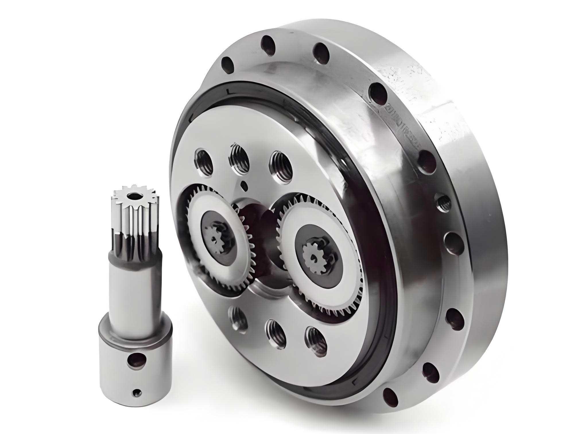
To initiate the reliability assessment, a transmission performance degradation test was conducted on RV reducers. Given that the typical lifespan under rated load is around 6,000 hours, an accelerated stress method was employed to expedite the process. This involved applying a load higher than the rated torque to the output end, ensuring that the failure modes remain consistent while shortening the test duration. The experimental setup consisted of a reciprocating swing test rig, where a drive motor controlled the input shaft of the RV reducer, causing the output to oscillate. An inertial load component was attached to simulate real-world operational stresses, with the load magnitude adjusted based on swing speed profiles and physical parameters to achieve an appropriate acceleration factor.
The test procedure was systematic: first, the initial transmission error of each RV reducer was measured; second, the reducers underwent reciprocating swing cycles under the specified load, with each complete swing from start to return counted as one cycle; third, at intervals of 300,000 cycles, the reducers were removed to measure the current transmission error; and fourth, this process was repeated until 1.2 million cycles were completed, resulting in degradation data at 300k, 600k, 900k, and 1.2M cycles. This data forms the foundation for the subsequent analysis, focusing on how the RV reducer’s performance evolves over time.
With the degradation data in hand, the next step involves modeling the performance decline. Degradation failure is common in mechanical systems, where performance gradually deteriorates until it reaches a predefined threshold $D_f$, at which point the component is considered failed. The general mathematical model for degradation can be expressed as:
$$ y = D(t, a, b) + \epsilon $$
Here, $y$ represents the measured performance data (transmission error in arcseconds), $t$ is the working time or number of cycles, $D(t, a, b)$ is the degradation model function with parameters $a$ and $b$, and $\epsilon$ denotes measurement error. Since physical degradation models are often elusive, empirical models are fitted to the data. Common models include linear, exponential, power function, logarithmic, Lloyd-Lipow, and composite exponential forms, as summarized in Table 1.
| Model Type | Expression |
|---|---|
| Linear Model | $y = a t + b$ |
| Exponential Model | $y = b e^{a t}$ |
| Power Function Model | $y = b t^{a}$ |
| Logarithmic Function Model | $y = a \ln t + b$ |
| Lloyd-Lipow Model | $y = a – b t$ |
| Composite Exponential Model | $y = e^{-b t} a$ |
To determine the optimal degradation model for the RV reducer, the collected transmission error data from six test units were fitted using the least squares method. The correlation coefficient $r$ between the experimental data and each model was computed to assess goodness-of-fit. The formula for $r$ is:
$$ r = \frac{\sum_{i=1}^{n} (x_i – \bar{x})(y_i – \bar{y})}{\sqrt{\sum_{i=1}^{n} (x_i – \bar{x})^2 \sum_{i=1}^{n} (y_i – \bar{y})^2}} $$
where $x_i$ are the time-series data (cycles), $y_i$ are the model-predicted values, and $\bar{x}$ and $\bar{y}$ are their respective means. A value of $|r|$ closer to 1 indicates stronger linear correlation and better fit. The results for all six RV reducer units are presented in Table 2, showcasing the correlation coefficients for each model.
| Model Type | Unit 1 | Unit 2 | Unit 3 | Unit 4 | Unit 5 | Unit 6 | Average |
|---|---|---|---|---|---|---|---|
| Linear Model | 0.9775 | 0.9846 | 0.9787 | 0.9614 | 0.9927 | 0.9769 | 0.9786 |
| Exponential Model | 0.9571 | 0.9833 | 0.9609 | 0.9189 | 0.9689 | 0.9541 | 0.9572 |
| Power Function Model | 0.9732 | 0.9616 | 0.9753 | 0.9887 | 0.9930 | 0.9735 | 0.9776 |
| Logarithmic Function Model | 0.9443 | 0.9153 | 0.9516 | 0.9876 | 0.9635 | 0.9419 | 0.9507 |
| Lloyd-Lipow Model | 0.8352 | 0.7793 | 0.8457 | 0.9234 | 0.8526 | 0.9341 | 0.8617 |
| Composite Exponential Model | 0.9773 | 0.9711 | 0.9791 | 0.9853 | 0.9962 | 0.9772 | 0.9807 |
From Table 2, the linear model exhibits the highest average correlation coefficient across all RV reducer units, indicating it best captures the degradation trend. Thus, for this RV reducer, the linear degradation model is selected as optimal. The fitted linear equations for each unit are summarized in Table 3, where $y$ is transmission error in arcseconds and $t$ is cycles.
| Unit Number | Fitted Linear Equation |
|---|---|
| 1 | $y = 1.7133 \times 10^{-5} t + 17.2249$ |
| 2 | $y = 1.7115 \times 10^{-5} t + 16.6008$ |
| 3 | $y = 1.4942 \times 10^{-5} t + 19.6406$ |
| 4 | $y = 1.5738 \times 10^{-5} t + 18.9193$ |
| 5 | $y = 1.8300 \times 10^{-5} t + 15.9628$ |
| 6 | $y = 1.7932 \times 10^{-5} t + 16.2797$ |
Using this linear model, the pseudo-failure life of each RV reducer can be estimated by extrapolating to a predefined failure threshold. For transmission error, a common threshold is set at $D_f = 50$ arcseconds. Solving $y = D_f$ in the linear equation $y = a t + b$ yields the pseudo-failure life $t_f$:
$$ t_f = \frac{D_f – b}{a} $$
Applying this to each RV reducer, the pseudo-failure lives in cycles are computed and presented in Table 4. These values represent the estimated number of cycles until the RV reducer’s transmission error degrades to the failure point, providing a basis for reliability analysis.
| Unit Number | Pseudo-Failure Life (cycles) |
|---|---|
| 1 | 1,912,937 |
| 2 | 1,951,379 |
| 3 | 2,031,753 |
| 4 | 1,974,870 |
| 5 | 1,859,866 |
| 6 | 1,880,417 |
With pseudo-failure life data available, the next phase involves fitting a lifetime distribution model to assess the overall reliability of the RV reducer population. The Weibull distribution is widely used in reliability engineering due to its flexibility in modeling various failure patterns. The three-parameter Weibull distribution is particularly suitable, as it includes a location parameter $\gamma$ to account for a minimum life threshold. Its probability density function (PDF) and cumulative distribution function (CDF) are given by:
$$ f(x) = \frac{\beta}{\alpha} \left( \frac{x – \gamma}{\alpha} \right)^{\beta – 1} e^{-\left( \frac{x – \gamma}{\alpha} \right)^\beta} $$
$$ F(x) = 1 – e^{-\left( \frac{x – \gamma}{\alpha} \right)^\beta} $$
where $\beta > 0$ is the shape parameter, $\alpha > 0$ is the scale parameter, and $\gamma$ is the location parameter. For the RV reducer, $x$ represents the pseudo-failure life in cycles. To estimate these parameters from the data, the maximum likelihood estimation (MLE) method is employed. The likelihood function $L(\alpha, \beta, \gamma)$ for $n$ data points is:
$$ L(\alpha, \beta, \gamma) = \prod_{i=1}^{n} \frac{\beta}{\alpha} \left( \frac{x_i – \gamma}{\alpha} \right)^{\beta – 1} e^{-\left( \frac{x_i – \gamma}{\alpha} \right)^\beta} $$
Taking the natural logarithm, we obtain the log-likelihood function:
$$ \ln L(\alpha, \beta, \gamma) = n \ln \frac{\beta}{\alpha} + (\beta – 1) \sum_{i=1}^{n} \ln \left( \frac{x_i – \gamma}{\alpha} \right) – \sum_{i=1}^{n} \left( \frac{x_i – \gamma}{\alpha} \right)^\beta $$
The parameters are estimated by solving the system of equations derived from setting the partial derivatives of $\ln L$ with respect to $\alpha$, $\beta$, and $\gamma$ to zero. This results in:
$$ \frac{\partial \ln L}{\partial \alpha} = -\frac{n}{\alpha} + \frac{\beta}{\alpha} \sum_{i=1}^{n} \left( \frac{x_i – \gamma}{\alpha} \right)^\beta = 0 $$
$$ \frac{\partial \ln L}{\partial \beta} = \frac{n}{\beta} + \sum_{i=1}^{n} \ln \left( \frac{x_i – \gamma}{\alpha} \right) – \sum_{i=1}^{n} \left( \frac{x_i – \gamma}{\alpha} \right)^\beta \ln \left( \frac{x_i – \gamma}{\alpha} \right) = 0 $$
$$ \frac{\partial \ln L}{\partial \gamma} = -(\beta – 1) \sum_{i=1}^{n} \frac{1}{x_i – \gamma} + \frac{\beta}{\alpha} \sum_{i=1}^{n} \left( \frac{x_i – \gamma}{\alpha} \right)^{\beta – 1} = 0 $$
Solving these equations analytically is complex, so numerical methods like the Newton-Raphson iteration are used. For the RV reducer data, applying MLE yields the estimated parameters: $\alpha = 118,187$, $\beta = 1.4057$, and $\gamma = 1,833,618$. Thus, the fitted PDF and CDF for the RV reducer’s lifetime are:
$$ f(t) = \frac{1.4057}{118,187} \left( \frac{t – 1,833,618}{118,187} \right)^{0.4057} e^{-\left( \frac{t – 1,833,618}{118,187} \right)^{1.4057}} $$
$$ F(t) = 1 – e^{-\left( \frac{t – 1,833,618}{118,187} \right)^{1.4057}} $$
The reliability function $R(t)$, which gives the probability that the RV reducer survives beyond time $t$, is then:
$$ R(t) = 1 – F(t) = e^{-\left( \frac{t – 1,833,618}{118,187} \right)^{1.4057}} $$
This function allows us to compute the reliability at any given number of cycles. For instance, the mean time to failure (MTTF) can be derived as the expected value of the distribution. For the three-parameter Weibull distribution, MTTF is given by:
$$ \text{MTTF} = \gamma + \alpha \Gamma\left(1 + \frac{1}{\beta}\right) $$
where $\Gamma(\cdot)$ is the gamma function. Plugging in the parameters for the RV reducer:
$$ \Gamma\left(1 + \frac{1}{1.4057}\right) \approx \Gamma(1.7113) \approx 0.910 $$
$$ \text{MTTF} \approx 1,833,618 + 118,187 \times 0.910 \approx 1,941,268 \text{ cycles} $$
This MTTF represents the average pseudo-failure life under the accelerated test conditions. To translate this into reliability metrics, we can evaluate $R(t)$ at specific points. For example, at $t = \text{MTTF} = 1,941,268$ cycles, the reliability of the RV reducer is:
$$ R(1,941,268) = e^{-\left( \frac{1,941,268 – 1,833,618}{118,187} \right)^{1.4057}} = e^{-\left( \frac{107,650}{118,187} \right)^{1.4057}} \approx e^{-(0.910)^{1.4057}} \approx e^{-0.876} \approx 0.416 $$
This indicates a reliability of approximately 41.6% at the mean life, which is typical for wear-out failures where reliability decreases over time. The reliability curve for the RV reducer, plotted using $R(t)$, shows a gradual decline as cycles increase, reflecting the degradation process.
To further elaborate on the methodology, it’s essential to discuss the assumptions and limitations. The linear degradation model for the RV reducer assumes a constant rate of increase in transmission error, which may hold true under steady operational conditions but could vary with different load profiles or environmental factors. Additionally, the accelerated testing approach assumes that the failure mechanisms remain unchanged under higher stress, which is valid if the acceleration factor is carefully calibrated. The use of the three-parameter Weibull distribution for the RV reducer accounts for a minimum life threshold, aligning with the idea that degradation only becomes significant after an initial period.
In practice, for RV reducers deployed in industrial robots, this reliability assessment framework can inform maintenance schedules and replacement strategies. By monitoring transmission error periodically, one can predict remaining useful life and plan interventions before failure occurs, thus minimizing downtime. The models derived here are specific to the tested RV reducers, but the approach can be generalized to other units by collecting similar degradation data.
Future work could involve expanding the sample size of RV reducers to enhance the statistical robustness of the estimates. Incorporating covariates such as load variations, temperature, or lubrication conditions into the degradation model could provide more nuanced reliability predictions. Moreover, validating the models with field data from actual RV reducer operations would strengthen their practical applicability.
In conclusion, this article has presented a comprehensive reliability assessment methodology for RV reducers based on transmission performance degradation data. Through accelerated testing, the linear degradation model was identified as optimal for the RV reducer, enabling pseudo-failure life estimation. Using maximum likelihood estimation, a three-parameter Weibull distribution was fitted to the lifetime data, yielding a reliability function that quantifies the RV reducer’s performance over time. The calculated MTTF and reliability values offer actionable insights for ensuring the durability and efficiency of RV reducers in robotic applications. By emphasizing key concepts like degradation modeling and statistical inference, this approach provides a valuable tool for engineers and researchers focused on enhancing the reliability of critical components like the RV reducer.