
The manufacturing of spiral bevel gears is a complex process that demands high precision to ensure optimal performance in power transmission systems, particularly in demanding applications like automotive differentials, aerospace actuators, and heavy industrial machinery. A critical post-machining operation for these gears is tooth crest chamfering. The sharp edges formed at the intersection of the tooth flank and the tooth crest are potential stress concentrators. Under dynamic loading conditions, influenced by manufacturing and assembly errors, these sharp corners can lead to premature failure mechanisms such as micro-cracking, pitting initiation, and noise generation. Therefore, chamfering these edges is not merely a finishing touch but a essential step to enhance gear life, reduce operational noise, and improve overall reliability. However, traditional chamfering methods for spiral bevel gears often face significant challenges related to efficiency, precision, and tool life, necessitating the exploration of more robust and economical techniques.
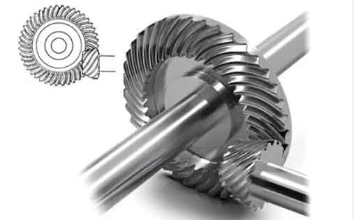
This article presents a comprehensive methodology for the chamfering of spiral bevel gears utilizing a standard disc cutter mounted on a conventional spiral bevel gear milling machine. The core objectives are to achieve simultaneous chamfering of both sides of a tooth space in a single pass, thereby improving efficiency; to leverage the longer cutting circumference of a disc cutter to enhance tool life compared to shaped tools like cone or pencil grinders; and to eliminate the need for costly, specialized chamfering equipment. The proposed method involves a systematic approach encompassing geometrical modeling, machining parameter calculation based on swept volume intersection, virtual simulation for parameter optimization, and shape error evaluation.
Geometrical Foundation and Modeling of Spiral Bevel Gears with Chamfer
The starting point for accurate chamfering is a precise digital model of the spiral bevel gear, inclusive of the desired chamfer feature. The tooth surface of a spiral bevel gear is typically composed of two primary zones: the active conjugate flank and the fillet or transition surface connecting the flank to the tooth bottom. The mathematical representation of these surfaces can be derived from the gear generation principles, often based on the Gleason or Klingelnberg systems.
The coordinates of discrete points on both the conjugate flank and the transition surface are calculated using established meshing theory and machine-tool setting equations. Let the position vector of a point on the generated gear surface be represented in the gear coordinate system \( S_g(X_g, Y_g, Z_g) \) as:
$$ \mathbf{r}_g = \mathbf{r}_g(u, \theta) $$
where \( u \) is a parameter along the tooth profile (often related to the cutter blade geometry) and \( \theta \) is the rotation parameter of the gear during generation. The surface normal \( \mathbf{n}_g \) is correspondingly calculated. These discrete point clouds for the concave (drive) and convex (coast) flanks, along with their respective fillets, serve as the foundational data.
This point cloud data is imported into a CAD or advanced simulation environment. Through interpolation and curve-fitting algorithms, cross-sectional profiles of a single tooth are reconstructed at various sections along the face width. A solid model of a single tooth is then created via a lofting operation through these profiles. The chamfer feature is explicitly added to this model by defining a chamfer width (e.g., 0.6 mm) at a specified angle (commonly 45°) along the tooth crest edges. Finally, a rotational pattern operation yields the complete three-dimensional model of the spiral bevel gear with chamfers. In this model, two key edge lines are defined for each side of a tooth space:
- Crest Line: The intersection curve between the chamfer surface and the original tooth crest cylindrical/conical surface.
- Flank Line: The intersection curve between the chamfer surface and the active tooth flank surface.
For a single tooth space, there are therefore four such guiding lines: crest and flank lines on both the concave and convex sides.
Machining Parameter Synthesis via Swept Volume Intersection
The central challenge is to determine the tool path for a disc cutter such that its cutting envelope simultaneously approximates all four guiding lines (two crest lines and two flank lines) of a tooth space. Perfect simultaneous contact is kinematically complex; therefore, an approximation method based on swept volumes is employed. The goal is to find a path for the disc cutter’s axis that minimizes the deviation from these ideal lines.
The fundamental idea is to use the guiding lines as trajectories to generate “theoretical” swept volumes of the disc cutter. By analyzing the intersection of these volumes, a compromise tool path can be derived. The step-by-step procedure is as follows:
- Model Extension: To ensure the calculated path covers the entire active tooth length, the single-tooth solid model is virtually extended beyond the nominal toe and heel regions along the lengthwise direction.
- Swept Volume Generation for Flank Lines: Using the concave and convex flank lines (\(L_{f1}\) and \(L_{f2}\)) as sweep paths, two cylindrical swept volumes (\(V_{f1}\) and \(V_{f2}\)) are created. The diameter \(d\) of these virtual cylinders equals the chosen disc cutter diameter. When \(d\) is sufficiently large, these two cylinders will intersect. The intersection generates two space curves. The curve farther from the gear body, denoted as \(C_f\), is selected. This curve \(C_f\) possesses a unique property: a cylinder of diameter \(d\) swept along it would be tangent to both original flank lines.
- Swept Volume Generation for Crest Lines: An identical process is applied to the two crest lines (\(L_{c1}\) and \(L_{c2}\)). They are used to generate swept volumes \(V_{c1}\) and \(V_{c2}\), whose intersection yields the distant space curve \(C_c\). A cylinder swept along \(C_c\) is tangent to both crest lines.
- Optimal Tool Path Determination: At this stage, we have two candidate tool axis paths: \(C_f\) (optimal for flank lines) and \(C_c\) (optimal for crest lines). The final tool path \(C_t\) is constructed as a weighted blend of these two to balance errors on the flank and crest sides. Both curves are discretized into \(n\) points (e.g., n=400). Let \( \mathbf{r}_{f}(i) \) and \( \mathbf{r}_{c}(i) \) be the position vectors of the \(i\)-th point on \(C_f\) and \(C_c\), respectively. The \(i\)-th point on the final tool path \(C_t\) is calculated as:
$$ \mathbf{r}_{t}(i) = \mu \cdot \mathbf{r}_{f}(i) + (1 – \mu) \cdot \mathbf{r}_{c}(i) $$
where \( \mu \) is a blending coefficient in the range [0, 1]. The disc cutter is then positioned with its geometric center on \( \mathbf{r}_{t}(i) \) and its axis of rotation aligned with the tangent vector to the path at that point, \( \mathbf{t}_{t}(i) \). By sequentially moving the cutter through all positions \( \mathbf{r}_{t}(i) \), the chamfering of the entire tooth space is accomplished in one continuous motion.
The machining parameters are thus defined by the disc cutter diameter \(d\), the number of discretization points \(n\), and the blending coefficient \( \mu \). The optimal values for \(d\) and \( \mu \) are not obvious and must be determined through analysis to minimize the resulting chamfer shape error.
Kinematic Transformation for Machine Tool Axes
To execute the calculated tool path \(C_t\) on a real spiral bevel gear milling machine, the continuous path must be converted into coordinated motions of the machine’s axes. A typical universal milling machine for spiral bevel gears features several programmable axes: linear axes (X, Y, Z) and rotational axes (A, B), often configured in a “workpiece tilting” type layout.
A coordinate transformation framework is established. Let the machine coordinate system \( S_m(O_m; X_m, Y_m, Z_m) \) have its origin \(O_m\) at a defined home position of the cutter center. The gear coordinate system \( S_g(O_g; X_g, Y_g, Z_g) \) is attached to the workpiece, with its origin \(O_g\) at the intersection of the gear axis and the B-axis rotation center. The vector from \(O_m\) to \(O_g\) is a constant machine offset \( \mathbf{d}_{off} \).
For any tool position defined by the center point \( \mathbf{r}_{t}(i) = (x_g, y_g, z_g)^T \) in \(S_g\) and the tool axis direction (unit tangent) \( \mathbf{t}_{t}(i) = (t_x, t_y, t_z)^T \) also in \(S_g\), we need to solve for the corresponding machine coordinates: rotations \( \theta_A, \theta_B \) and translations \( d_X, d_Y, d_Z \).
The condition that the tool axis aligns with the machine’s spindle direction (commalong \(Z_m\)) after rotations gives:
$$ \mathbf{R}_B(\theta_B) \cdot \mathbf{R}_A(\theta_A) \cdot \begin{bmatrix} t_x \\ t_y \\ t_z \end{bmatrix}_{S_g} = \begin{bmatrix} 0 \\ 0 \\ 1 \end{bmatrix}_{S_m} $$
where \( \mathbf{R}_A \) and \( \mathbf{R}_B \) are rotation matrices about the A and B axes respectively. This equation solves for \( \theta_A \) and \( \theta_B \).
The condition that the tool center coincides with the programmed point in the machine frame gives:
$$ \begin{bmatrix} d_X \\ d_Y \\ 0 \\ 1 \end{bmatrix} = \mathbf{T}_{trans}(0,0,d_Z) \cdot \mathbf{T}_{trans}(\mathbf{d}_{off}) \cdot \mathbf{T}_{rot}(\theta_B) \cdot \mathbf{T}_{rot}(\theta_A) \cdot \begin{bmatrix} x_g \\ y_g \\ z_g \\ 1 \end{bmatrix} $$
where \( \mathbf{T}_{rot} \) and \( \mathbf{T}_{trans} \) are homogeneous transformation matrices. This equation is solved for the linear axis positions \( d_X, d_Y, \) and \( d_Z \). By performing this inverse kinematics calculation for every discretized point along \(C_t\), the NC code for the chamfering operation is generated.
Virtual Simulation and Shape Error Evaluation
Given the complexity of the geometry and the approximative nature of the tool path calculation, a virtual simulation environment is crucial for validating the method and optimizing the parameters \(d\) and \( \mu \). A dynamic simulation environment is constructed within a finite element or multi-body dynamics software capable of Boolean operations. This environment includes models of the machine tool structure, the rotating disc cutter, and the spiral bevel gear blank.
The simulation proceeds in a discrete manner, replicating the NC code. At each simulation step corresponding to a machine interpolation cycle, the cutter model is positioned according to the calculated axes positions \( (\theta_A, \theta_B, d_X, d_Y, d_Z) \). A Boolean subtraction operation is then performed, removing the material volume occupied by the cutter from the gear blank. This process is repeated sequentially until the cutter has traversed the entire path, resulting in a simulated chamfered gear. This virtual machining process allows for the testing of multiple parameter sets \( (d, \mu) \) without physical waste.
To quantitatively assess the quality of the chamfer, a shape error metric is defined. On the simulated gear, measurement planes are created at several sections along the face width (e.g., at the toe, middle, and heel, and intermediate points, totaling 10 measurement locations per tooth space). At each location, two key distances are measured on the simulated chamfer:
- Crest Distance (\(D_c\)): The distance from a defined reference point on the original sharp crest (before chamfering) to the point where the machined chamfer surface intersects the remaining crest surface.
- Flank Distance (\(D_f\)): The distance from the same reference point to the point where the machined chamfer surface intersects the active tooth flank.
These measured distances are compared to the nominal or theoretical distances (\(D_{c0}\) and \(D_{f0}\)) obtained from the perfect CAD model of the chamfer. The shape error at a measurement location \(k\) can be defined in absolute terms:
$$ e_{abs}^k = \max( |D_c^k – D_{c0}^k|, |D_f^k – D_{f0}^k| ) $$
or in relative terms:
$$ e_{rel}^k = \max\left( \frac{|D_c^k – D_{c0}^k|}{D_{c0}^k}, \frac{|D_f^k – D_{f0}^k|}{D_{f0}^k} \right) \times 100\% $$
The overall chamfer shape error for a parameter set is taken as the maximum value of \(e_{abs}^k\) or \(e_{rel}^k\) across all measurement locations. The optimal machining parameters \( (d_{opt}, \mu_{opt}) \) are those that minimize this overall shape error.
Comprehensive Application Example
The following example demonstrates the complete procedure for a spiral bevel pinion. The basic gear design and machine settings for generating the pinion are first established.
| Parameter | Value | Parameter | Value |
|---|---|---|---|
| Number of Teeth | 17 | Face Width | 75 mm |
| Pitch Cone Angle | 21.084° | Outer Cone Distance | 253.529 mm |
| Face Cone Angle | 24.068° | Whole Tooth Depth (outer) | 18.413 mm |
| Root Cone Angle | 20.473° | Hand of Spiral | Left |
| Setting Item | Concave Side | Convex Side |
|---|---|---|
| Cutter Radial Distance (mm) | 214.459 | 197.571 |
| Cutter Tilt Angle (°) | 66.454 | 74.731 |
| Machine Center to Back (mm) | 45.712 | 45.712 |
| Sliding Base Setting (mm) | -2.009 | 6.719 |
| Ratio of Roll | 3.425 | 3.114 |
| Cutter Point Radius (mm) | 238.901 | 223.988 |
| Pressure Angle (°) | -26 / 16 (Duplex) |
A nominal chamfer width of 0.6 mm at 45° is specified. The disc cutter thickness is set to 10 mm. The number of path discretization points is fixed at \(n=400\). A parameter study is conducted by varying the disc cutter diameter \(d\) and the blending coefficient \( \mu \). Three cutter diameters are evaluated: 34 mm, 36 mm, and 38 mm. For each diameter, \( \mu \) is varied from 0 to 1 in steps of 0.1, resulting in 33 distinct parameter combinations. For each combination \((d, \mu)\), the tool path \(C_t\) is calculated, the NC code is generated via kinematic transformation, and a virtual machining simulation is performed. The absolute and relative shape errors are measured according to the defined protocol.
| Cutter Diameter \(d\) (mm) | Optimal \(\mu\) for Min. Absolute Error | Minimum Absolute Error \(e_{abs}^{min}\) (mm) | Optimal \(\mu\) for Min. Relative Error | Minimum Relative Error \(e_{rel}^{min}\) (%) |
|---|---|---|---|---|
| 34 | 0.3 | 0.157 | 0.4 | 16.5 |
| 36 | 0.4 | 0.130 | 0.5 | 14.8 |
| 38 | 0.5 | 0.141 | 0.6 | 15.9 |
The results clearly indicate that a disc cutter diameter of \(d = 36\) mm yields the best performance. With a blending coefficient of \(\mu = 0.4\), it achieves the smallest absolute shape error of 0.13 mm. With \(\mu = 0.5\), it achieves the smallest relative error of 14.8%. The choice between these two optimal \(\mu\) values can be made based on whether absolute dimensional tolerance or proportional accuracy is more critical for the specific application of the spiral bevel gears. The virtual simulation successfully identifies workable and optimized parameters, demonstrating the feasibility of the entire methodology.
Discussion and Advantages of the Proposed Method
The research outlines a systematic engineering approach for chamfering spiral bevel gears. The use of a simple disc cutter is a significant advantage. Compared to formed-profile tools or small-diameter end mills, the disc cutter presents a much longer segment of its cutting edge to the workpiece during the operation. This distributes wear over a larger area, drastically reducing the rate of tool degradation, increasing tool life, and minimizing downtime for tool changes. This is a major cost-saving and efficiency-boosting factor in a production environment.
Furthermore, the method is designed for implementation on existing spiral bevel gear milling machines. By simply installing a disc cutter holder and utilizing the machine’s standard multi-axis CNC capabilities to execute the calculated path, the need for a dedicated, special-purpose chamfering machine is eliminated. This represents a substantial reduction in capital investment and floor space requirements.
The core algorithm based on swept volume intersection and linear blending provides a robust and computationally efficient way to generate a practical tool path. While it produces an approximation, the subsequent virtual simulation and error minimization loop ensure that the approximation error is controlled and reduced to acceptable levels for most industrial applications of spiral bevel gears. The shape error metrics provide clear, quantitative criteria for accepting or further optimizing a set of machining parameters.
Potential areas for future refinement include the development of more advanced tool path blending strategies beyond a simple linear combination, perhaps using optimization algorithms to directly minimize the sum of squared deviations from all four guiding lines. Additionally, integrating real-time tool wear monitoring and compensation into the process could further enhance the consistency of the chamfer quality over long production runs for spiral bevel gears.
Conclusion
This article has detailed a complete and practical methodology for performing tooth crest chamfering on spiral bevel gears using a standard disc cutter. The process integrates precise geometric modeling of the spiral bevel gear with chamfer, a novel tool path generation technique based on the intersection of virtual swept volumes, inverse kinematics for machine tool control, and virtual simulation for parameter optimization and validation. The method successfully addresses key industrial challenges: it enables efficient simultaneous dual-side chamfering in a single pass, significantly extends tool life due to the favorable geometry of the disc cutter, and leverages existing gear milling machinery, avoiding the cost of specialized equipment. By employing the simulation-based optimization loop to minimize chamfer shape error, the method ensures high precision. This combination of efficiency, economy, and precision makes the disc-cutter-based approach a highly viable and advantageous solution for the post-machining treatment of high-value spiral bevel gears across various manufacturing sectors.