
Hypoid gears are widely used in vehicle drive axles, marine propulsion, and aerospace transmissions because of their high load-carrying capacity, smooth meshing, and compact design. In the manufacturing process, however, tooth surface errors are inevitably introduced by machine tool inaccuracies, cutter wear, thermal deformation, and elastic deflections. These errors directly affect the contact pattern, vibration, noise, and fatigue life of the gear pair. To reduce the number of trial cuts and improve the efficiency of error correction, I systematically study the generation principle of hypoid gears, establish a high-precision five-axis CNC machining simulation platform, and propose an improved linear regression based tooth surface error correction method. This paper is organized around the following key contributions: mathematical modeling of the tooth surface, virtual machining simulation, sensitivity analysis of machine settings, and a flexible correction strategy that minimizes the number of adjusted settings while satisfying the tolerance requirements.
1. Introduction
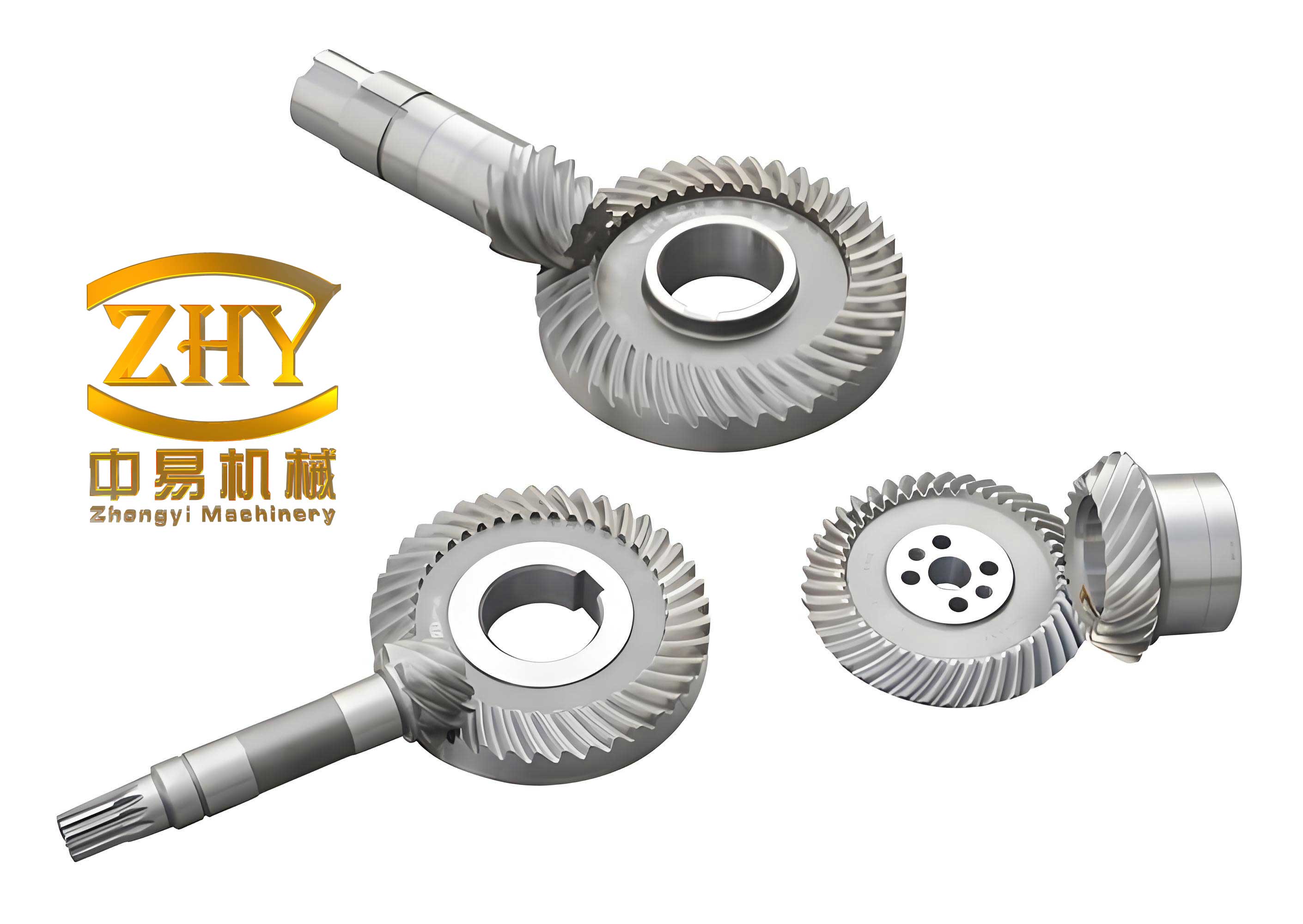
Hypoid gears belong to a special family of spiral bevel gears in which the axes of the pinion and gear are offset in space. This offset enables a larger spiral angle, which improves the meshing contact ratio and reduces the minimum number of pinion teeth. In commercial vehicle rear axles, hypoid gears are the primary reducing and torque-transferring components, and their tooth surface accuracy is one of the most important factors that determine the axle noise and durability.
Traditional mechanical cradle-type gear generators, such as the widely used No. 116 style machines, rely on complex linkages to generate the tooth surface. The machine settings include the cutter tilt angle, swivel angle, radial distance, initial cradle angle, vertical offset, machine center to back, sliding base, and root angle of the work head. Because of the many coupled adjustment parameters, hand-tuning the machine settings to compensate for tooth surface errors is tedious and requires repeated trial cuts with coordinate measurements.
With the advancement of CNC technology, modern six-axis five-linkage hypoid gear generators have replaced mechanical machines in many production facilities. However, due to the high cost of full CNC generators, a majority of small- and medium-sized enterprises still rely on older mechanical machines or retrofitted CNC versions. It is therefore meaningful to develop an equivalent five-axis machining center that can reproduce the kinematics of a traditional cradle-type generator, and to create a virtual simulation environment for studying the tooth surface error correction methods before physical cutting.
The objective of this work is to propose a flexible tooth surface error correction method that can determine the minimal set of machine settings to be adjusted in order to reduce the measured tooth surface errors to an acceptable level. I first derive the mathematical model of the tooth surface for both the generated pinion and the formate gear. Then, I construct a virtual five-axis CNC machining platform based on the equivalent kinematics of a traditional machine. Next, I analyze the influence of each machine setting on the resulting tooth surface errors and build a sensitivity matrix. Finally, I improve the conventional linear regression approach for selecting the correction parameters and validate the proposed method through both virtual cutting experiments and physical cutting tests.
2. Mathematical Model of Hypoid Gear Tooth Surface
2.1 Machining Methods and Fundamental Principles
Two basic manufacturing methods are commonly used for hypoid gears: face-milling (also known as completing or single-indexing process) and face-hobbing (continuous indexing process). For the face-milling method, a cup-shaped cutter head with a group of inside and outside blades generates one tooth slot at a time, and then the work piece is indexed to the next slot. The tooth lengthwise curvature is a circular arc; therefore this method is suitable for tapered gears which are conventional in automotive axles. In contrast, face-hobbing uses a continuous indexing process where the cutter head and work piece rotate in a timed relationship, producing an epicycloid tooth profile.
Within the face-milling method, the gear can be produced either by the forming process or by the generation process. In the forming process, the gear tooth surface is the exact mirror of the cutter blades; the cradle remains stationary, and only the cutter head rotates while being fed into the work blank. This method is highly productive for large gears with pitch angles greater than about 70°, so it is widely used for ring gears (the large hypoid gear). The small pinion is usually generated by a rolling process in which a virtual crown gear or a tapered generating gear is formed by the cutter head and the cradle rotation. The pinion tooth surface is generated as the envelope of the cutting blades.
According to the gearing theory, the generation process is equivalent to the meshing between the generating gear (the cutter head and cradle) and the work gear. The relative motion satisfies the fundamental equation of meshing:
$$ \mathbf{n} \cdot \mathbf{v}^{(12)} = 0, $$
where \(\mathbf{n}\) is the common unit normal vector at a contact point, and \(\mathbf{v}^{(12)}\) is the relative velocity between the generating surface and the generated surface at that point.
2.2 Cutter Head Model
The cutter head is a key element that directly generates the tooth surface. In this study, a face-milling cutter with a nominal radius \(r_0\) is considered. The cutting edges are straight lines in the axial section, having a pressure angle \(\alpha\). For a blade point defined by the depth coordinate \(s\) along the cutting edge and the angular position \(\theta\) around the cutter axis, the position vector of the cutting edge in the cutter coordinate system \(S_c\) can be written as
$$ \mathbf{r}_c(s,\theta) = \begin{bmatrix} (R \mp s \sin \alpha)\cos\theta \\ (R \mp s \sin \alpha)\sin\theta \\ -s \cos\alpha \\ 1 \end{bmatrix}, \quad R = r_0 \mp \frac{W}{2}, $$
where \(W\) is the blade point width (cutter blade offset), the upper sign refers to the outside blade and the lower sign to the inside blade. The unit normal vector to the cutting surface is
$$ \mathbf{n}_c(\theta) = \begin{bmatrix} \cos\alpha\cos\theta \\ \cos\alpha\sin\theta \\ \mp \sin\alpha \\ 0 \end{bmatrix}. $$
2.3 Tooth Surface of the Formate Gear (Large Gear)
For the formate gear, the cutter head is installed on the machine without tilt and swivel. The coordinate systems include the cutter coordinate system \(S_c\), the machine coordinate system \(S_m\), and the work gear coordinate system \(S_1\). The transformation from the cutter to the work gear is obtained by successive translations and rotations:
$$ \mathbf{r}_1(s_1,\theta_1) = M_{1m} M_{mc} \mathbf{r}_c(s_1,\theta_1), $$
where
$$ M_{mc} = \begin{bmatrix} 1 & 0 & 0 & H \\ 0 & 1 & 0 & V \\ 0 & 0 & 1 & -\Delta B\\ 0 & 0 & 0 & 1 \end{bmatrix}, \qquad M_{1m} = \begin{bmatrix} \cos\gamma_{m1} & 0 & \sin\gamma_{m1} & -\Delta A \\ 0 & 1 & 0 & 0 \\ -\sin\gamma_{m1} & 0 & \cos\gamma_{m1} & 0 \\ 0 & 0 & 0 & 1 \end{bmatrix}. $$
Here \(H\) and \(V\) are the horizontal and vertical machine offsets, \(\Delta B\) is the sliding base, \(\gamma_{m1}\) is the machine root angle, and \(\Delta A\) is the machine center to back distance.
2.4 Tooth Surface of the Generated Pinion (Tilted Head Process)
For the pinion, the cutter head can be tilted and swiveled to realize a tapered generating gear. The complete transformation chain includes several intermediate coordinate systems. The fundamental machine settings are listed in Table 1.
| Parameter | Symbol | Concave side | Convex side |
|---|---|---|---|
| Cutter blade radius | \(r_0\) | 150 mm | 150 mm |
| Blade pressure angle | \(\alpha\) | 14° | 35° |
| Blade edge radius | \(\rho\) | 2.20 mm | 2.20 mm |
| Machine root angle | \(\gamma_m\) | -2.00° | -4.00° |
| Horizontal setting | \(\Delta A\) | -4.75 mm | 6.34 mm |
| Sliding base | \(\Delta B\) | 23.69 mm | 39.90 mm |
| Vertical offset | \(E_m\) | 26.91 mm | 34.61 mm |
| Cutter tilt angle | \(i\) | 9.54230° | 11.61026° |
| Cutter swivel angle | \(j\) | 261.233° | 281.417° |
| Radial distance | \(S_R\) | 127.39791 mm | 134.83515 mm |
| Initial cradle angle | \(q_0\) | 68.04821° | 58.19035° |
| Roll ratio | \(Ratio\) | 5.82073 | 6.44114 |
The tooth surface of the pinion is expressed as
$$ \mathbf{r}_2(s_2,\theta_2,\phi) = M_{2f} M_{fe} M_{ed} M_{dm} M_{mc} M_{ct} \mathbf{r}_c(s_2,\theta_2), $$
where \(\phi\) is the work gear rotation angle, and the transformations are derived from the machine kinematics. By applying the meshing equation in the machine coordinate system, one obtains
$$ f(s_2,\theta_2,\phi) = \mathbf{n}^{(2)} \cdot \mathbf{v}^{(12)} = 0, $$
which, after eliminating \(s_2\), reduces the tooth surface to a two-parameter family:
$$ \mathbf{r}_2(\theta_2,\phi) = \mathbf{h}(\theta_2,\phi). $$
2.5 Discretization of the Tooth Surface and 3D Model Construction
To visualize the tooth surface and to generate a three-dimensional model, the tooth surface is discretized into a grid of \(5 \times 9\) points. The two-dimensional projection of the tooth surface in the axial plane is divided along the tooth height and face width directions. The coordinates of the four corners \(A,B,C,D\) are first computed from the blank geometry
$$ \begin{aligned} x_A &= R_c \cos\delta – h_a \sin\delta, \quad r_A = R_c \sin\delta + h_a \cos\delta, \\ x_B &= R_c \cos\delta + h_f \sin\delta, \quad r_B = R_c \sin\delta – h_f \cos\delta, \end{aligned} $$
and then all interior points are obtained by linear interpolation along the boundaries. For each point, a nonlinear system is solved in MATLAB using the fsolve function to determine the surface parameters \((\theta,\phi)\), and the 3D coordinates are computed.
The discrete point clouds for the concave and convex surfaces are imported into CATIA. A closed tooth slot volume is created by combining the flank surfaces with the root cone, face cone, and toe/heel planar boundaries. After filling this volume, the slot is patterned around the gear axis and subtracted from the blank to obtain the complete gear model. The resulting 3D solid models of the pinion and gear are shown in the following figures. The discrete coordinates of the gear tooth flank points are listed in Appendix A of the original thesis.
3. Five-Axis CNC Machining Simulation Platform
3.1 Kinematic Equivalence Between Traditional Cradle Generator and a Five-Axis Machining Center
A five-axis CNC machining center is designed to replicate the motion of a traditional cradle-type hypoid gear generator. The configuration consists of three linear axes (X, Y, Z) and two rotary axes (A, B) under the workpiece, plus an additional spindle axis C for the cutter head. The X and Y linear axes replace the eccentric crank and cradle angular positioning, the Z axis provides the depth feed, the A axis performs the work spindle rotation for generating and indexing, and the B axis swings the work head to reproduce the machine root angle.
To convert the traditional machine settings to the five-axis CNC commands, I derive the cutter head position and orientation vectors in the workpiece coordinate system through both the traditional machine chain and the CNC machine chain. Equating these two representations yields the following expressions for the CNC axes:
$$ \begin{cases} A = \dfrac{\phi}{Ratio} + \arctan\!\left(\dfrac{\sin i \sin(q+j)}{\sin i \sin \gamma_m \cos(q+j) – \cos i \cos\gamma_m}\right), \\ B = \arcsin\!\left(\cos i \sin\gamma_m + \sin i \cos\gamma_m \cos(q+j)\right), \end{cases} $$
and the linear axes are given by
$$ \begin{cases} X = \dfrac{a}{\cos B} – \sin B\left(b\sin A + c\cos A + a\tan B\right), \\ Y = \dfrac{b}{\cos A} + \left(a\tan B – b\sin A – c\cos A – a\tan B \sin^2 B – a\sin B\cos B\right)\tan A, \\ Z = -\left(b\sin A\cos B + c\cos A\cos B + a\sin B\right), \end{cases} $$
where \(a,b,c\) are the components of the cutter position vector in the workpiece frame, and \(q = q_0 + \phi_c\) is the cradle angle at each instant.
3.2 Generation of G-code Program
The continuous rotation of the cradle and workpiece in a mechanical generator is replaced by a sequence of discrete cutter locations in the CNC machine. For each rolling position \(\phi_c\), the corresponding five-axis coordinates are computed using the above equations. A G-code program is then generated with a linear interpolation motion (G01) between successive positions. The procedure consists of the following steps:
| Block | Function |
|---|---|
| M03, M08 | Start spindle rotation, coolant on |
| G00 X… Y… Z… A… B… | Rapid traverse to the initial cutting position |
| G01 X… Y… Z… A… B… | Linear interpolation for one rolling sequence |
| G00 Z… | Retract after completing one tooth slot |
| G01 A… (incremented by \(360/z\)) | Index to the next tooth |
| M05, M02 | Stop spindle, end of program |
In the actual program, the rolling step size is set to 0.1° or smaller to ensure sufficient accuracy.
3.3 VERICUT Simulation and Its Limitations
I built a virtual machine model in VERICUT by importing the three-dimensional CAD models of the base, linear axes, rotary axes, spindle, and workhead. The tool library is created with the appropriate inside and outside cutter blades. After running the G-code program, a complete gear tooth form is generated. The automatic comparison function of VERICUT is then used to inspect the machined model against the design model. The simulation results show that the maximum deviation is approximately 0.02 mm, which arises from tessellation errors in the STL representation. Such accuracy is insufficient for studying the tooth surface error correction because the sensitivity coefficients require the machining error to be controlled below 1 μm. Therefore, I chose to implement a more precise virtual cutting simulation in CATIA by using the VBA macro programming environment.
3.4 High-Precision Cutting Simulation in CATIA
The CATIA-based simulation uses the same machine setting transformations to position the cutter head and the work blank. The cutter head model is built directly from the blade parameters, and the gear blank is drawn according to the blank dimensions. The simulation flow is shown in Figure below:
The process is as follows:
- Initialize the blank and cutter in the default position.
- Apply the work blank adjustments: horizontal setting \(\Delta A\), machine root angle \(\gamma_m\), vertical offset \(E_m\), and sliding base \(\Delta B\).
- Apply the cutter head adjustments: for the formate gear, only the horizontal and vertical cutter positions are used; for the generated pinion, the tilt, swivel, radial distance, eccentric angle, and cradle angle are used.
- For each rolling position, rotate the work blank by an incremental angle and the cradle by the corresponding incremental angle according to the roll ratio.
- Perform a Boolean subtraction operation to remove the material swept by the cutter from the blank at each step.
- Repeat the rolling sequence and then index to the next tooth slot.
I implemented this algorithm using the CATIA VBA interface. The cutter and blank are transformed continuously, and a Boolean operation is executed at each step. To reduce the computation time, the pinion flank is generated on the convex side with a rolling step of 0.1°, which gives a maximum simulated tooth surface deviation of 0.0011 mm relative to the theoretical surface. By reducing the step sizes to 0.01° for the cradle and 0.0644° for the work piece, the maximum deviation further decreases to 0.0003 mm. The high-precision simulation platform is therefore suitable for generating error tooth surfaces for the correction method research.
4. Tooth Surface Error Correction Method Based on Improved Linear Regression Analysis
4.1 Tooth Surface Error Definition and Decomposition
Tooth surface error is defined as the signed normal distance from a theoretical surface point to the actual manufactured surface. A positive error means the actual surface lies outside the theoretical surface in the normal direction. The measured error includes both the index error (tooth spacing error) and the profile error. The index error causes the entire tooth flank to rotate around the gear axis by a constant angular offset. This offset does not affect the flank topology and should be removed before the profile error is used for correction.
Let \(P_1\) be the midpoint of the theoretical flank, and \(P_2\) the corresponding midpoint of the measured flank. The angular offset \(\Delta\phi\) that aligns \(P_1\) with \(P_2\) is found by solving
$$ y_{P_2}\cos\Delta\phi + z_{P_2}\sin\Delta\phi = y_{P_1}. $$
After subtracting the index error, the corrected actual flank coordinates are used to compute the normal deviations at each grid point.
4.2 Sensitivity Coefficient Matrix
The tooth surface position vector depends on the machine settings vector \(\mathbf{k}\) and the surface parameters:
$$ \mathbf{r} = \mathbf{r}(\theta,\phi,\mathbf{k}), \quad \mathbf{k} = [\Delta A, \Delta B, E_m, S_R, i, j, \gamma_m, Ratio]^T. $$
By differentiating the position vector and taking the dot product with the surface unit normal \(\mathbf{n}\), one obtains a linearized relation between the tooth surface error \(\mathbf{e}\) and the machine setting deviations \(\Delta\mathbf{k}\):
$$ \mathbf{e} = S \Delta\mathbf{k}, $$
where \(S\) is the \(45 \times 8\) sensitivity matrix. The entry \(s_{ij}\) denotes the change of the error at the \(i\)-th grid point caused by a unit change of the \(j\)-th machine setting. In practice, I compute \(S\) numerically by applying a small perturbation to each setting and measuring the corresponding tooth surface deviation. For instance, a +0.1 mm change of the vertical offset \(E_m\) of the pinion produces errors in the range of -0.0211 mm to 0.018 mm on the convex side, and -0.0167 mm to 0.0167 mm on the concave side.
The influence of each machine setting on the tooth surface error is summarized in Table 3, where the comprehensive influence coefficient \(E_j\) is defined as the sum of the absolute deviations at all 45 grid points divided by the parameter change magnitude:
$$ E_j = \frac{\sum_{i=1}^{45} |e_{ij}|}{\Delta k_j}. $$
| Machine setting | Convex side (\(E_j\)) | Concave side (\(E_j\)) |
|---|---|---|
| Horizontal setting \(\Delta A\) | 1.651 | 2.247 |
| Sliding base \(\Delta B\) | 0.657 | 1.840 |
| Vertical offset \(E_m\) | 3.146 | 2.777 |
| Angular position of cutter \(q_0\) | 0 | 0 |
| Radial distance \(S_R\) | 5.121 | 5.813 |
| Tilt angle \(i\) | 8.015 | 8.136 |
| Swivel angle \(j\) | 0.617 | 0.522 |
| Machine root angle \(\gamma_m\) | 3.500 | 2.848 |
| Roll ratio \(Ratio\) | 84.5 | 91.4 |
It is clear that the roll ratio has the strongest influence on the pinion tooth surface error, followed by the tilt angle, radial distance, and machine root angle. The angular position of the cutter has virtually no effect.
4.3 Basic Correction Method Using Least Squares
Given the measured tooth surface error vector \(\mathbf{e}_m\), the machine setting correction vector \(\Delta\mathbf{k}\) can be obtained by solving the over-determined linear system
$$ S\Delta\mathbf{k} = \mathbf{e}_m, $$
in the least squares sense. The normal equations are
$$ S^T S \Delta\mathbf{k} = S^T \mathbf{e}_m. $$
However, using all eight machine settings as correction parameters often yields large but unrealistic corrections because of the coupling among the settings. In production, adjusting too many settings is time-consuming and may destroy the previously established contact pattern. Therefore, it is preferable to select only a small number of machine settings that have the strongest correlation with the measured error pattern.
4.4 Traditional Linear Regression Approach
The traditional linear regression method selects the correction parameters one by one. First, a univariate linear regression is performed between each sensitivity column \(s_j\) and the measured error \(\mathbf{e}_m\). The coefficient of determination \(R^2\) is computed for each setting. The setting with the largest \(R^2\) is chosen as the first correction parameter. If the residual sum of squares is still larger than the tolerance, a bivariate regression is performed by pairing the first parameter with each of the remaining parameters, and the one that gives the largest \(R^2\) is selected as the second parameter. The process continues until the residual meets the required accuracy.
Although this stepwise method works, it does not guarantee the globally optimal solution. A parameter that has the highest \(R^2\) in the univariate regression may not be part of the best pair in the bivariate regression. Consequently, the method may require more correction parameters than necessary.
4.5 Improved Linear Regression Approach
To overcome the limitation of the stepwise procedure, I improve the selection strategy as follows. Instead of fixing the previously chosen parameters, I evaluate all possible combinations of \(n\) parameters from the full set of \(m\) candidates. For each combination, I perform an \(n\)-variate linear regression and compute the corresponding \(R^2\). The combination with the largest \(R^2\) is chosen as the optimal correction parameter set for that order. The procedure is:
- Set the maximum permissible number of correction parameters (e.g., 3).
- For \(n=1\) to \(n_{max}\), enumerate all \(C_m^n\) combinations of machine settings.
- For each combination, solve the linear least squares problem to determine the parameter corrections and compute the residual \(RSS\).
- Select the combination that gives the smallest \(RSS\) (or equivalently, the largest adjusted \(R^2\)).
- If the residual is within the required tolerance, stop; otherwise increase \(n\) and repeat.
| Method | Selected parameters | \(R^2\) | Residual max (μm) |
|---|---|---|---|
| Traditional bivariate | \(\Delta A, \gamma_m\) | 0.9626 | — |
| Improved bivariate | \(E_m, \gamma_m\) | 0.9719 | — |
| Traditional trivariate | \(\Delta A, \gamma_m, Ratio\) | 0.9804 | 6.6 |
| Improved trivariate | \(\Delta A, \Delta B, Ratio\) | 0.9857 | — |
| Improved bivariate (best) | \(E_m, \gamma_m\) | 0.9719 | 8.4 |
The improved method is more flexible because it can find the globally optimal parameter combination of each dimension. Moreover, it provides the user with several acceptable combinations that meet the tolerance, allowing the process engineer to choose those settings that are easier to adjust on a specific machine.
4.6 Virtual Correction Simulation
To verify the improved method, I introduced a deliberate error in the cutter blade radius by +0.2 mm and in the blade pressure angle by +0.2° on the concave side of the pinion. The resulting tooth surface error was simulated in the CATIA cutting platform. The measured maximum error was 70.3 μm and the average absolute error was 26.2 μm. The correction parameters were then computed by three methods: (i) least squares using all settings, (ii) traditional stepwise linear regression, and (iii) improved regression with exhaustive combinatorial search. The resulting corrections are listed in Table 5.
| Parameter | Least squares | Traditional regression | Improved regression |
|---|---|---|---|
| \(\Delta A\) (mm) | +0.4264 | +0.2532 | — |
| \(\Delta B\) (mm) | -0.2239 | — | — |
| \(E_m\) (mm) | -0.1348 | — | -0.4613 |
| \(S_R\) (mm) | -0.0265 | — | — |
| \(i\) (°) | +0.0061 | — | — |
| \(j\) (°) | +0.4114 | — | — |
| \(\gamma_m\) (°) | +0.0575 | +0.1159 | +0.4154 |
| \(Ratio\) | -0.0059 | -0.0060 | — |
After applying the corrections to the virtual machine and re-cutting the gear, the remaining tooth surface errors were measured. With the traditional method, three parameters were required to bring the maximum residual error below 6.6 μm. With the improved method, only two parameters (\(E_m\) and \(\gamma_m\)) were sufficient to reduce the maximum error to 8.4 μm, and the average absolute error to 2.32 μm. This confirms that the improved method reduces the number of correction parameters while achieving essentially the same accuracy as the traditional three-parameter approach.
5. Experimental Verification on a Physical Gear Generator
5.1 Measurement Equipment and Procedure
To validate the proposed method in a real production environment, I used a CNC hypoid gear generator and a coordinate measuring machine (CMM) equipped with a rotary table. The gear pair used in the experiment has the same basic design as the simulation example: a 6-tooth pinion and 37-tooth gear with a module of 8.65 mm, a pressure angle of 22.5°, an offset of 30 mm, and a face width of about 48 mm for the pinion.
Before measuring, the theoretical tooth surface was converted into a grid of \(5 \times 9\) points in the CMM coordinate system. The gear was aligned by fixing the gear axis along the CMM vertical axis, and the measurement origin was set at the gear pitch apex. I used a “split measurement” strategy: starting from the tooth surface midpoint, the probe traverses toward the toe and heel sides separately. This strategy reduces the rotary table angular errors compared to a sequential zigzag path. Three non-consecutive teeth were measured, and the average of the three measurements was used as the actual tooth surface error.
| Parameter | Pinion | Gear |
|---|---|---|
| Number of teeth | 6 | 37 |
| Module (mm) | 8.65 | |
| Pressure angle (°) | 22.5 | |
| Offset (mm) | 30 (below) | |
| Mean spiral angle (°) | 48 | 35.783 |
| Hand of spiral | Left | Right |
| Face width (mm) | 47.91 | 43 |
| Shaft angle (°) | 90 | |
| Pitch cone angle (°) | 10.1 | 79.667 |
| Face cone angle (°) | 15.233 | 80.317 |
| Root cone angle (°) | 9.467 | 74.417 |
5.2 Initial Tooth Surface Errors
The first trial cut was performed using the original machine settings from Table 1. The measured tooth surface errors on the convex and concave flanks are presented in Figure below. The convex side shows a maximum absolute error of 106.9 μm and an average absolute error of 30.76 μm. The concave side shows a maximum absolute error of 110.6 μm and an average absolute error of 31.6 μm. The dominant error pattern is diagonal, meaning that the error changes from toe to heel and from root to tip simultaneously. This suggests that a combination of machine settings capable of producing a diagonal correction is required.
5.3 Correction Calculation Using the Improved Method
Using the improved linear regression selection procedure, the optimal correction parameter sets were determined for both sides. For the convex side, the selected parameters were the vertical offset \(E_m\), the swivel angle \(j\), and the machine root angle \(\gamma_m\). For the concave side, the selected parameters were the radial distance \(S_R\), the swivel angle \(j\), and the roll ratio. The calculated corrections are given in Table 7.
| Side | Parameter | Original value | Corrected value | Correction |
|---|---|---|---|---|
| Convex | \(E_m\) (mm) | 34.6100 | 34.4188 | -0.1912 |
| \(j\) (°) | 281.4170 | 283.1732 | +1.7562 | |
| \(\gamma_m\) (°) | -4.0000 | -3.6655 | +0.3345 | |
| Concave | \(S_R\) (mm) | 127.39791 | 127.23881 | -0.1591 |
| \(j\) (°) | 261.2330 | 258.9299 | -2.3031 | |
| \(Ratio\) | 5.82073 | 5.83093 | +0.0102 |
Before the actual re-cutting, the theoretical residual errors were computed by applying the corrections to the sensitivity model. For the convex side, the predicted maximum residual error was 9.7 μm and the average was 2.769 μm. For the concave side, the predicted maximum residual error was 9.5 μm and the average was 3.36 μm.
5.4 Measurement After Correction
The corrected machine settings were entered into the CNC generator, and a second gear was cut. The tooth surface errors were measured again using the same CMM method. The measured errors after correction are shown in Figure below. The convex side exhibited a maximum absolute error of 8.2 μm and an average absolute error of 3.376 μm. The concave side exhibited a maximum absolute error of 7.6 μm and an average absolute error of 3.62 μm. Both flanks satisfy the production tolerance of 10 μm maximum error.
| Side | Initial max error (μm) | Initial mean error (μm) | Predicted max residual (μm) | Corrected max error (μm) | Corrected mean error (μm) |
|---|---|---|---|---|---|
| Convex | 106.9 | 30.76 | 9.7 | 8.2 | 3.376 |
| Concave | 110.6 | 31.60 | 9.5 | 7.6 | 3.620 |
Figure shows the comparison of the measured errors at the 45 grid points for both flanks. The corrected errors closely follow the theoretically predicted residual curve, which validates the accuracy of the sensitivity matrix and the correction algorithm. The small difference between the predicted and measured residuals is attributed to measurement repeatability (about ±1 μm) and to the fact that the actual machine setting adjustments cannot be realized with arbitrary precision.
6. Conclusion
In this thesis, I have systematically studied the CNC machining simulation and tooth surface error correction method for hypoid gears. The main contributions and conclusions are summarized as follows.
- I established the mathematical models for both the formate gear and the generated pinion tooth surfaces. By combining the cutter head model, coordinate transformations, and the equation of meshing, the accurate tooth surface point coordinates were computed. The discrete points were then used to construct the solid three-dimensional models in CATIA.
- I developed a five-axis CNC machining simulation platform on the basis of the kinematic equivalence with a traditional cradle-type generator. The platform was implemented in VERICUT and CATIA. The CATIA-based simulation, using VBA-controlled Boolean subtraction, achieved a tooth surface error of less than 0.0011 mm, which is sufficiently accurate for the sensitivity analysis in correction research.
- I analyzed the influence of each machine setting on the tooth surface error. The roll ratio, tilt angle, radial distance, vertical offset, and machine root angle are the most influential parameters, whereas the angular cutter position has no effect on the flank error.
- I proposed an improved linear regression analysis based correction method. Instead of the stepwise addition of parameters, the improved method exhaustively searches all combinations of a given number of parameters and chooses the combination with the highest coefficient of determination. The simulation results demonstrated that the improved method requires only two correction parameters to achieve the same error reduction that the traditional method achieves with three parameters.
- I conducted physical cutting experiments and CMM measurements on a real hypoid gear generator. After the first trial cut, the maximum error exceeded 100 μm. By applying the corrections computed with the improved method, the maximum tooth surface error was reduced to below 8.2 μm, and the average absolute error was reduced to about 3.4–3.6 μm, meeting the required tolerance.
Future work will focus on extending the correction method to consider high-order tooth surface deviations, exploring the coupling effects among machine settings, and developing a closed-loop automated correction system that can directly communicate with modern CNC generators. The proposed method provides a practical and efficient solution for reducing trial-cut iterations in hypoid gear production.