
In the field of power transmission, especially within automotive drive axles, hypoid gears are renowned for their superior performance characteristics, including high load capacity, smooth operation, and the ability to accommodate significant offset between non-intersecting axes. The accurate prediction and analysis of their tooth contact patterns under load are critical for ensuring durability, minimizing noise, and optimizing efficiency. This work presents a comprehensive methodology for the tooth contact analysis (TCA) of hypoid gears by synergistically integrating analytical modeling techniques with advanced finite element simulation. The goal is to overcome the limitations of purely analytical TCA, which often involves complex curvature calculations and can be prone to numerical instability, while providing a more realistic and intuitive visualization of the three-dimensional loaded contact area.
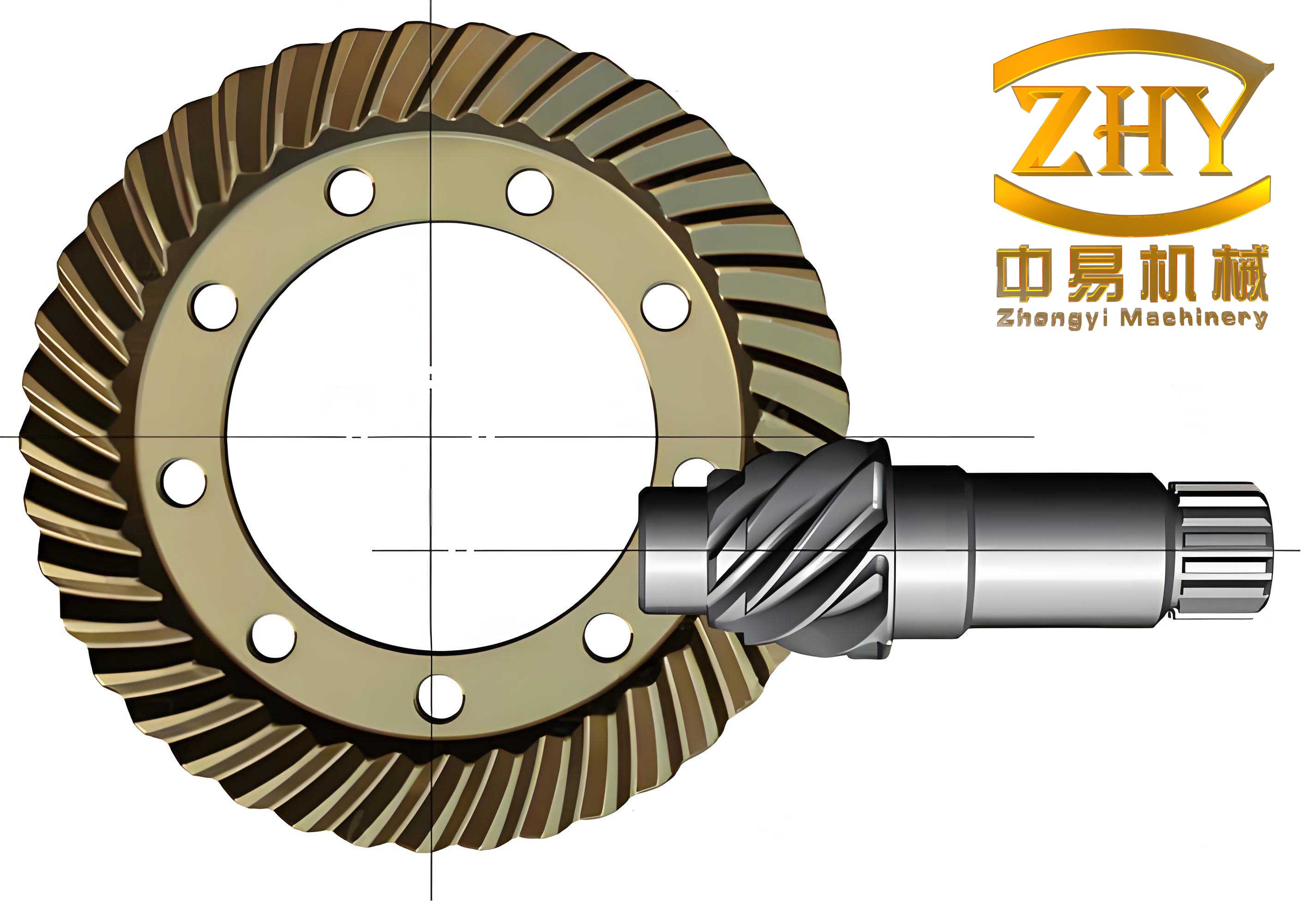
The foundational step in any gear analysis is the precise mathematical description of the tooth flanks. For hypoid gears manufactured via the HFT (Hyperboloidal Form Tool) method, the process begins with defining the cutter geometry. The coordinate system attached to the cutter head, $S_t (X_t, Y_t, Z_t)$, is established where the cutting edges of the inside and outside blades are defined. A point on the blade surface is parameterized by variables $u_k$ and $\theta_k$, where $k = g, p$ denotes the inside (generating) and outside (producing) blades, respectively. The surface equation and unit normal vector for the cutter in $S_t$ are given by:
$$
\mathbf{r}_t(u_k, \theta_k) = \begin{bmatrix}
(r_k + u_k \sin \alpha_k) \cos \theta_k \\
(r_k + u_k \sin \alpha_k) \sin \theta_k \\
-u_k \cos \alpha_k \\
1
\end{bmatrix}, \quad \mathbf{n}_t(\theta_k) = \begin{bmatrix}
-\cos \alpha_k \cos \theta_k & -\cos \alpha_k \sin \theta_k & \sin \alpha_k
\end{bmatrix}^T
$$
Here, $r_k$ is the cutter point radius and $\alpha_k$ is the blade pressure angle. The complex relative motion between the cutter and the workpiece in HFT machining is captured through a series of coordinate transformations involving machine settings such as the machine root angle $\gamma_m$, sliding base setting $X_b$, radial setting $S_{r1}$, angular setting $q_1$, workpiece offset $E_{m1}$, and the ratio of roll $R_b$. The final pinion tooth surface $\Sigma_1$ and its unit normal in the workpiece coordinate system $S_1$ are derived through the transformation chain:
$$
\mathbf{r}_1(u_k, \theta_k, \phi) = \mathbf{M}_{1d}\mathbf{M}_{dh}\mathbf{M}_{hs}\mathbf{M}_{sm}\mathbf{M}_{mc}\mathbf{M}_{cj}\mathbf{M}_{jt} \mathbf{r}_t(u_k, \theta_k)
$$
$$
\mathbf{n}_1(u_k, \theta_k, \phi) = \mathbf{L}_{1d}\mathbf{L}_{dh}\mathbf{L}_{hs}\mathbf{L}_{sm}\mathbf{L}_{mc}\mathbf{L}_{cj}\mathbf{L}_{jt} \mathbf{n}_t(\theta_k)
$$
The parameter $\phi$ is the cradle rotation angle, linked to the workpiece rotation $\varphi$ via the roll ratio ($\phi = R_b \varphi$). The gear tooth surface, typically generated by a formate (non-generated) process, is a special case of this model with specific settings like roll ratio set to zero.
With the mathematical models for both pinion and gear tooth flanks established, the unloaded meshing condition can be analyzed. The core of analytical TCA is solving the system of equations that enforce contact and tangency between the two surfaces in a fixed coordinate system $S_a$. The conditions require that at the point of contact, the position vectors and the unit normals of both surfaces coincide:
$$
\mathbf{r}_{a1}(u_1, \theta_1, \varphi_1) = \mathbf{r}_{a2}(u_2, \theta_2, \varphi_2)
$$
$$
\mathbf{n}_{a1}(u_1, \theta_1, \varphi_1) = \mathbf{n}_{a2}(u_2, \theta_2, \varphi_2)
$$
This system consists of five independent scalar equations with six unknowns ($u_1, \theta_1, \varphi_1, u_2, \theta_2, \varphi_2$). By prescribing the pinion rotation angle $\varphi_1$ as an input, the system can be solved numerically for the remaining five variables, tracing the path of contact across the tooth flank. A key output from this analysis is the transmission error (TE), which quantifies the deviation from perfectly conjugate motion. It is calculated as:
$$
\Delta \varphi_2 = (\varphi_2 – \varphi_2^{(0)}) – \frac{z_1}{z_2} (\varphi_1 – \varphi_1^{(0)})
$$
where $z_1$ and $z_2$ are the numbers of teeth, and $\varphi_1^{(0)}, \varphi_2^{(0)}$ are the initial contact angles at a reference point. While analytical TCA efficiently provides the transmission error curve and the potential contact path, determining the instantaneous contact ellipse traditionally requires computing the principal curvatures and directions of both surfaces at the contact point—a mathematically intensive process. This is where the fusion with the Finite Element Method (FEM) offers a powerful alternative for contact zone visualization.
The process transitions from pure analytics to numerical geometry and simulation. First, a dense point cloud representing the tooth surface is calculated from the mathematical model using a numerical sampling algorithm. These points are then imported into CAD software (e.g., Siemens NX) to construct a precise, watertight 3D solid model of the hypoid gear pair. For efficient and accurate finite element analysis, a single tooth segment of both the pinion and gear is often extracted and prepared with partitions to facilitate a structured hexahedral mesh, which is generally more robust for contact problems. This prepared geometry is exported for simulation.
The finite element analysis workflow, implemented in a solver like ABAQUS, consists of three main stages: Pre-processing, Solution, and Post-processing. A summary of the key parameters for a representative hypoid gear pair used in this study is provided in the tables below.
| Parameter | Pinion | Gear |
|---|---|---|
| Number of Teeth | 8 | 39 |
| Hand of Spiral | Left | Right |
| Shaft Angle | 90° | 90° |
| Offset | 35 mm (below) | 35 mm (below) |
| Module | 6.283 mm | 6.283 mm |
| Spiral Angle at Ref. | 50.24° | 31.37° |
| Pressure Angle | 22.5° | 22.5° |
| Face Width | 44.4 mm | 38 mm |
| Machine Setting | Pinion (Convex Side) | Gear (Concave Side) |
|---|---|---|
| Cutter Radius | 120.91 mm | 115.86 mm |
| Cutter Blade Angle | -14° | -22.5° |
| Cutter Tilt Angle (j) | 12.11° | 0° |
| Cutter Swivel Angle (i) | 331.83° | 0° |
| Radial Setting (Sr1) | 104.3279 mm | 109.058 mm |
| Ratio of Roll (Rb) | 4.702215 | 0 (Formate) |
In Pre-processing, the gear models are assembled with the correct spatial relationship (offset and shaft angle). Material properties such as density, Young’s modulus, and Poisson’s ratio for alloy steel are assigned. A critical step is mesh generation; a fine, structured hexahedral mesh is applied to the tooth contact regions to accurately resolve contact stresses, while coarser elements can be used elsewhere for computational efficiency. Contact pairs are defined between the pinion and gear tooth flanks, typically using a surface-to-surface discretization with a finite sliding formulation. A reasonable friction coefficient may be defined. Boundary conditions are applied to simulate real operating conditions: the gear is fixed in all degrees of freedom except rotation about its axis, and the pinion is driven by applying a prescribed torque or rotation while constraining its other motions.
During the Solution phase, a static, general step is used to simulate the loaded condition. The nonlinear equations stemming from the contact are solved incrementally. The primary field output of interest is the contact pressure (CPRESS) or stress distribution on the tooth flanks at each increment or frame of the analysis.
The final and crucial stage is Post-processing for contact zone visualization. The loaded tooth contact area is not a single ellipse but the aggregation of all instantaneous contact ellipses throughout the meshing cycle under load. A custom Python script is developed to process the ABAQUS results database (.odb file). The script operates by reading the contact stress field output for all frames of the analysis. For each element on the contact surface, it identifies the maximum contact stress value experienced over the entire meshing cycle. This maximum value is then mapped back onto the element in a final, single visualization step. This process effectively compresses the time-history of contact into a single image showing the complete three-dimensional area where contact stresses occurred, thus representing the loaded tooth contact pattern. This method bypasses the analytical curvature calculation entirely, leveraging the solver’s ability to compute actual deformations and contact pressures.
To validate the proposed fused methodology, a case study was performed on the hypoid gear pair defined in Tables 1 and 2. First, the analytical component was verified. The transmission error curve was calculated using a custom MATLAB program implementing the equations described earlier. The result showed a parabolic-like TE function with an amplitude of approximately 28 micro-radians. This result was in excellent agreement with the output from a commercial gear design software (Gleason CAGE), which reported a TE amplitude of 28.5 micro-radians. This close correlation validates the correctness of the mathematical surface generation and the unloaded TCA algorithm.
Subsequently, the 3D gear models were created and subjected to Finite Element Analysis. The FEA model, after applying a representative load, yielded the instantaneous contact ellipses at various mesh positions. The Python post-processing script was then executed to compile these into the final loaded contact pattern. The resulting contact area for the gear concave side was observed to be located in the mid-to-inner region of the tooth flank, exhibiting a slightly diagonal orientation—a typical and desirable pattern for hypoid gears to avoid edge loading.
For further verification, this FEA-derived contact pattern was compared with the results from a dedicated, industry-standard gear analysis software suite, MASTA. Under similar load conditions, MASTA predicted a contact area with comparable shape, size, and location on the tooth flank. The strong visual and qualitative agreement between the independent FEM workflow and MASTA’s internal contact algorithms provides substantial confidence in the proposed fused approach.
The ultimate validation came from physical manufacturing and testing. The gear set was ground on a hypoid grinder using the calculated machine settings. The tooth surfaces were measured via coordinate measurement to ensure conformance to the theoretical design. Finally, the gear pair was run on a rolling tester (e.g., Gleason Tester) under a light load (40 Nm). The observed contact pattern on the gear concave side from the physical test showed remarkable consistency with the pattern predicted by the finite element simulation. Both displayed similar shape, orientation, and position on the tooth flank. This experimental correlation confirms not only the accuracy of the tooth surface model but also the practical validity of using finite element analysis, post-processed with cycle-maximum stress mapping, as a reliable method for predicting the loaded contact behavior of hypoid gears.
In conclusion, this research demonstrates an effective and robust methodology for the tooth contact analysis of hypoid gears by fusing analytical and finite element techniques. The analytical method provides an efficient and accurate calculation of fundamental unloaded performance metrics like transmission error and the path of contact. The finite element method, enhanced with a specialized post-processing script to aggregate instantaneous contact stresses over a mesh cycle, successfully predicts the three-dimensional loaded contact area without the need for complex analytical curvature derivations. The results from this fused approach show excellent agreement with both specialized commercial software predictions and physical rolling tests, establishing it as a credible and comprehensive tool for the design and performance evaluation of high-performance hypoid gear drives in automotive and other industrial applications.