
Throughout my graduate research, I focused on the establishment of a precise mathematical model for herringbone gear tooth surfaces and the development of corresponding measurement and error evaluation methods. Herringbone gears are widely used in high-speed and heavy-load transmission systems due to their excellent load-carrying capacity and self-balanced axial thrust. However, because of their complex geometric structure, creating an accurate tooth surface model and determining suitable measurement strategies remain challenging tasks. In this work, I systematically derived the tooth surface equations based on involute helical gear theory, implemented three-dimensional simulations using MATLAB, analyzed the principal gear errors according to national standards, developed a LabVIEW-based evaluation system, and finally validated the theoretical models through coordinate measuring machine (CMM) experiments. This article presents the entire methodology, the derived formulas, the key data tables, and the verification results.
1. Introduction and Background
Gears are fundamental components in mechanical equipment, providing reliable power transmission with high efficiency and long service life. Among all gear types, involute cylindrical gears are the most widely used due to their relatively simple geometry and ease of manufacturing. Herringbone gears, which can be regarded as a combination of two helical gears with opposite helix angles on the same gear blank, inherit all the advantages of helical gears while eliminating the axial thrust through self-balancing. This unique feature makes herringbone gears particularly suitable for applications in marine propulsion, aerospace transmissions, and heavy industrial machinery.
Despite their importance, the research on herringbone gears has lagged behind that on spur or single helical gears. The primary difficulties lie in the accurate description of the three-dimensional tooth surface and the complexity of measuring the tooth profile, helix, and pitch deviations. In my research, I addressed these difficulties by first establishing a rigorous coordinate system and deriving the parametric equations of the herringbone gear tooth surface. I then focused on the definition and computation of the main gear errors, including tooth profile deviation, helix deviation, and pitch deviation, following the guidelines of the ISO and Chinese national standards. Finally, I carried out practical measurements using a three-coordinate measuring machine, which proved the correctness and feasibility of the proposed methods.
The significance of this research can be summarized as follows:
- It provides a complete mathematical foundation for the digital modeling of herringbone gears.
- It offers practical formulas for calculating tooth profile, helix, and pitch deviations from coordinate measurement data.
- It demonstrates the integration of MATLAB computation and LabVIEW software for gear error evaluation, which can be extended to other complex gear types.
2. Mathematical Modeling of the Herringbone Gear Tooth Surface
2.1 Basic Parameters
A herringbone gear is essentially formed by two helical gears with the same tooth number, module, and pressure angle, but with opposite helix angles. Consequently, all the basic parameters of a helical gear apply, with the distinction between normal and transverse planes being essential. Table 1 lists the basic parameters and their calculation formulas that I used in the modeling process.
| Parameter | Symbol | Formula or Value |
|---|---|---|
| Normal module | \(m_n\) | Standard value |
| Transverse module | \(m_t\) | \(m_t = m_n / \cos\beta\) |
| Normal pressure angle | \(\alpha_n\) | \(\alpha_n = 20^\circ\) (standard) |
| Transverse pressure angle | \(\alpha_t\) | \(\sin\alpha_t = \sin\alpha_n / \cos\beta\) |
| Pitch circle diameter | \(d\) | \(d = m_t z\) |
| Base circle diameter | \(d_b\) | \(d_b = d \cos\alpha_t\) |
| Helix angle at pitch circle | \(\beta\) | Generally \(8^\circ\) to \(20^\circ\) |
| Base helix angle | \(\beta_b\) | \(\tan\beta_b = \tan\beta \cos\alpha_t\) |
| Addendum | \(h_a\) | \(h_a = h_a^* m_n\) |
| Dedendum | \(h_f\) | \(h_f = (h_a^* + c^*) m_n\) |
| Tip circle diameter | \(d_a\) | \(d_a = d + 2h_a\) |
| Root circle diameter | \(d_f\) | \(d_f = d – 2h_f\) |
| Transverse circular pitch | \(p_t\) | \(p_t = \pi m_t\) |
| Normal circular pitch | \(p_n\) | \(p_n = \pi m_n\) |
In my experiments, I used a herringbone gear with the parameters shown in Table 2. These parameters were used throughout the modeling and measurement process.
| Parameter | Symbol | Value |
|---|---|---|
| Normal module | \(m_n\) | 3.456811 mm |
| Number of teeth | \(z\) | 19 |
| Addendum coefficient | \(h_a^*\) | 1 |
| Clearance coefficient | \(c^*\) | 0.25 |
| Helix angle | \(\beta\) | 16.6772° |
| Pressure angle | \(\alpha\) | 22.5° |
| Face width | \(b\) | 30 mm (for model); 60 mm (for measurement) |
2.2 Involute Equation
The tooth profile of a herringbone gear is based on the involute of a circle. As shown in the standard involute construction, a straight line rolls without slipping on a base circle of radius \(r_b\). The locus of a point on this line is an involute. For an arbitrary point \(K\) on the involute, the polar coordinates \((r_k, \theta_k)\) satisfy the following equations:
\[
r_k = \frac{r_b}{\cos\alpha_k}
\]
\[
\theta_k = \tan\alpha_k – \alpha_k = \operatorname{inv}\alpha_k
\]
where \(\alpha_k\) is the pressure angle at point \(K\). Converting to Cartesian coordinates with the base circle center at the origin and the start point on the \(x\)-axis, I obtained:
\[
\begin{cases}
x_k = r_b \cos\varphi_k + r_b \varphi_k \sin\varphi_k \\
y_k = r_b \sin\varphi_k – r_b \varphi_k \cos\varphi_k
\end{cases}
\]
where \(\varphi_k = \theta_k + \alpha_k = \tan\alpha_k\) is the roll angle. This formulation was the starting point for describing the three-dimensional tooth surface.
2.3 Right Tooth Surface Equation of a Helical Gear
For a helical gear, the involute curves are generated by a plane that rolls on the base cylinder, while the generating line is inclined by the base helix angle \(\beta_b\). Figure 1 illustrates the formation of an involute helicoid.
To describe the complete tooth surface, I established a workpiece coordinate system with the gear axis as the \(Z\)-axis. For the right flank of the first tooth, a point \(P_{1Rjz}\) on the surface can be expressed as:
\[
\begin{cases}
X_{1Rjz} = r_b \cos(\theta_z + \varphi_{1Rj}) + r_b \varphi_{1Rj} \sin(\theta_z + \varphi_{1Rj}) – r_b \sin\theta_z \cos\varphi_{1Rj} \\
Y_{1Rjz} = r_b \sin(\theta_z + \varphi_{1Rj}) – r_b \varphi_{1Rj} \cos(\theta_z + \varphi_{1Rj}) – r_b \cos\theta_z \cos\varphi_{1Rj} \\
Z_{1Rjz} = \pm r_b \cot\beta_b \cdot \theta_z
\end{cases}
\]
In the above equations, \(\varphi_{1Rj}\) is the roll angle of the end-section involute at the point where it crosses the \(XOY\) plane, and \(\theta_z\) is the angular rotation of the generatrix along the helix. The \(\pm\) sign accounts for the two halves of the herringbone gear (positive \(Z\) for one helical direction, negative \(Z\) for the opposite direction).
For the \(i\)-th tooth, the right flank point is obtained by rotating the first-tooth point around the \(Z\)-axis by the angular pitch:
\[
\theta_i = \frac{2\pi}{z_0}(i-1) \quad (i=1,2,\dots,z_0)
\]
\[
P_{iRjz} = A_z^{-1}(\theta_i) P_{1Rjz}
\]
with the rotation matrix
\[
A_z(\theta_i) =
\begin{bmatrix}
\cos\theta_i & -\sin\theta_i & 0 \\
\sin\theta_i & \cos\theta_i & 0 \\
0 & 0 & 1
\end{bmatrix}
\]
2.4 Left Tooth Surface Equation
The left flank of a tooth is symmetric to the right flank with respect to a plane passing through the gear axis and the midpoint of the chordal tooth thickness. In the transverse plane, if the symmetry line is \(c: y = kx\), then the slope \(k\) can be determined from the angular tooth thickness. For a given tooth, the relation between a point on the right flank and the corresponding point on the left flank is given by a mirror transformation matrix \(V\):
\[
P_{1Ljz} = V \cdot P_{1Rjz}
\]
\[
V =
\begin{bmatrix}
\frac{k^2-1}{k^2+1} & \frac{2k}{k^2+1} & 0 \\
\frac{2k}{k^2+1} & \frac{1-k^2}{k^2+1} & 0 \\
0 & 0 & 1
\end{bmatrix}
\]
where \(k = -\tan(\varphi_f + \alpha_f)\). Here \(\varphi_f\) is the half angular tooth thickness on the pitch circle and \(\alpha_f\) is the pressure angle at the pitch circle. The same transformation applies at any height along the tooth surface because the symmetry property is identical for all transverse sections.
2.5 Complete Herringbone Gear Tooth Surface
A herringbone gear is composed of two identical helical gears mirrored with respect to the \(XOY\) plane. Therefore, the complete tooth surface equation can be obtained by using the positive or negative value of \(Z_{1Rjz}\) in the right flank equation. The final parametric representation for the \(i\)-th tooth, right flank, at the \(j\)-th point on the positive or negative \(Z\)-axis is:
\[
\begin{cases}
X_{iRjz} = r_b \cos(\theta_i \pm \theta_z + \varphi_{1Rj}) + r_b \varphi_{1Rj} \sin(\theta_i \pm \theta_z + \varphi_{1Rj}) – r_b \sin(\theta_i \pm \theta_z) \cos\varphi_{1Rj} \\
Y_{iRjz} = r_b \sin(\theta_i \pm \theta_z + \varphi_{1Rj}) – r_b \varphi_{1Rj} \cos(\theta_i \pm \theta_z + \varphi_{1Rj}) – r_b \cos(\theta_i \pm \theta_z) \cos\varphi_{1Rj} \\
Z_{iRjz} = \pm r_b \cot\beta_b \cdot \theta_z
\end{cases}
\]
Similarly, the left flank coordinates are obtained by applying the mirror matrix \(V\) and the rotation matrix \(A_z(\theta_i)\).
2.6 Numerical Simulation
Using MATLAB, I implemented the derived equations to compute the coordinates of points on the herringbone gear tooth surface. A program was written to sweep the involute profile along the helix angle and to mirror it for both halves of the gear. Table 3 summarizes the simulation parameters and the resulting coordinate ranges.
| Parameter | Value | Remarks |
|---|---|---|
| Base radius \(r_b\) | \(r_b = d_b/2\) | Calculated from parameters |
| Roll angle range \(\varphi\) | From \(\varphi_{root}\) to \(\varphi_{tip}\) | Determined by base and tip circles |
| Helix rotation range \(\theta_z\) | \(-b\tan\beta_b/(2r_b)\) to \(+\) same value | Depends on face width \(b\) |
| Number of teeth simulated | 1 or 19 | Single-tooth and full-gear options |
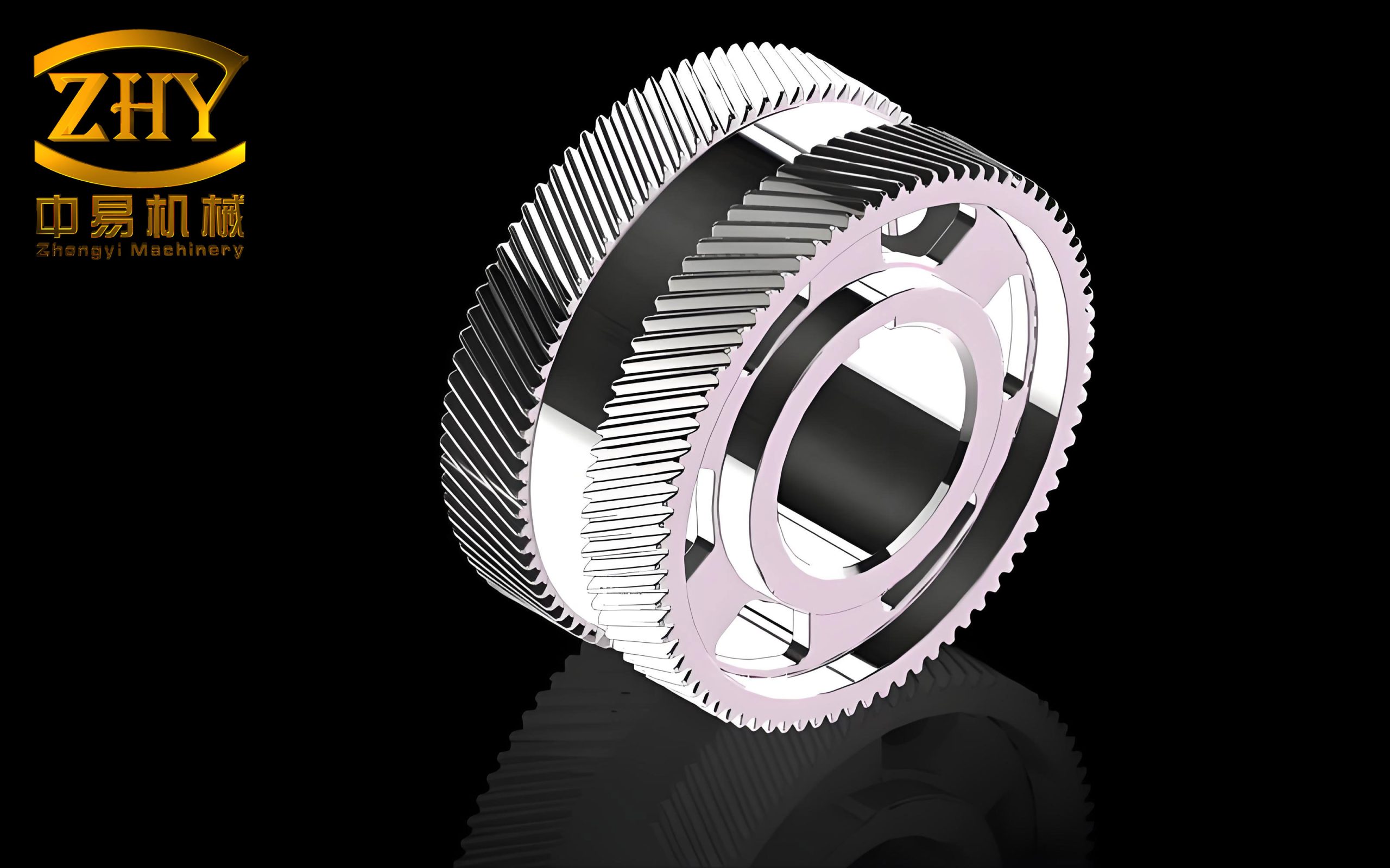
The three-dimensional simulation confirmed that the tooth surface is a smooth involute helicoid. Figure 1 shows the rendered herringbone gear tooth surface from the simulation software. The left and right flanks are correctly mirrored, and the two helical halves meet exactly at the mid-plane, demonstrating the correctness of the derived equations.
3. Error Analysis of Herringbone Gears
Gear errors directly influence transmission performance. Based on the Chinese national standard GB/T 10095.1-2001, the most important errors that must be checked are the tooth profile deviation, helix deviation, and pitch deviation. In this section, I explain the definitions and present the computational methods for these deviations using coordinate measurement data.
3.1 Tooth Profile Deviation
The tooth profile deviation is defined in the transverse plane, normal to the involute profile. Let \(P_i(x_i, y_i)\) be a measured point on the actual tooth flank. The polar radius and pressure angle at this point are:
\[
r_i = \sqrt{x_i^2 + y_i^2}
\]
\[
\alpha_i = \arccos\left(\frac{r_b}{r_i}\right)
\]
The polar angle of the point is:
\[
\phi_i = \arctan\left(\frac{y_i}{x_i}\right)
\]
The theoretical roll angle of the design involute passing through point \(P_i\) is:
\[
\theta_i = \tan\alpha_i – \alpha_i
\]
If the actual tooth profile is identical to the theoretical one but slightly rotated by a small angle \(\varepsilon\), then the measured point would satisfy:
\[
\phi_i + \theta_i = \varepsilon + \omega_i
\]
where \(\omega_i\) is the roll angle of the actual tooth profile at the base circle. The deviation of \(\omega_i\) from its mean can be obtained from:
\[
\Delta \omega_i = \phi_i + \theta_i – \varepsilon
\]
Since \(\varepsilon\) is constant for a given flank, the maximum and minimum values of \(\Delta\omega_i\) over all measured points provide the angular width that contains the actual profile. Converting this angular difference to a linear value in the normal direction gives the tooth profile total deviation:
\[
\Delta f_\alpha = r_b (\Delta\omega_{\max} – \Delta\omega_{\min}) \cos\beta
\]
After substituting the expressions, the final formula becomes:
\[
\Delta f_\alpha = r_b \left[ \arctan\left(\frac{y_1}{x_1}\right) + \tan\alpha_1 – \alpha_1 – \arctan\left(\frac{y_2}{x_2}\right) – \tan\alpha_2 + \alpha_2 \right] \cos\beta
\]
For the left flank, the sign in front of the roll angle changes accordingly. If \(m\) teeth are measured, the gear tooth profile total deviation is:
\[
F_\alpha = \max\left(\Delta f_{\alpha 1}, \Delta f_{\alpha 2}, \dots, \Delta f_{\alpha m}\right)
\]
Table 4 gives a sample of the measured tooth profile deviation calculation for the tested herringbone gear.
| Tooth | Flank | Point | \(\phi_i\) (rad) | \(\omega_i\) (rad) | \(\Delta f_\alpha\) (mm) |
|---|---|---|---|---|---|
| 1 | Left | 1 | 1.4773 | 1.4734 | 0.0139 |
| 1 | Left | 2 | 1.4879 | 1.4734 | |
| 1 | Left | 3 | 1.5014 | 1.4731 | |
| 1 | Left | 4 | 1.5175 | 1.4730 | |
| 1 | Left | 5 | 1.5357 | 1.4731 | |
| 4 | Right | 1 | 0.0643 | 0.0681 | 0.0081 |
| 4 | Right | 2 | 0.0534 | 0.0678 | |
| 4 | Right | 3 | 0.0396 | 0.0679 | |
| 4 | Right | 4 | 0.0235 | 0.0679 | |
| 4 | Right | 5 | 0.0054 | 0.0680 |
From the processed data, the tooth profile total deviation of the tested herringbone gear was \(F_\alpha = 0.0174\) mm.
3.2 Helix Deviation
The helix deviation is defined on the pitch cylinder as the distance between two design helix lines that exactly contain the actual helix trace, measured in the transverse plane. Since the herringbone gear is composed of two helical gears, the helix deviation is essentially the helix line deviation. To measure it, I used the three-dimensional coordinates of points on the tooth flank at the pitch circle. Let \(P_i(x_i, y_i, z_i)\) be the measured points. The angular position of each point with respect to the gear axis is:
\[
\theta_i = \arctan\left(\frac{y_i}{x_i}\right)
\]
The increment of the angle between two consecutive points is:
\[
\Delta\theta_i = \theta_i – \theta_{i-1}
\]
The corresponding arc length on the pitch circle is:
\[
\Delta W_i = r \Delta\theta_i
\]
where \(r\) is the pitch circle radius. According to the helix geometry, the theoretical angular increment corresponding to the axial displacement \(\Delta Z_i\) is:
\[
\Delta W_{t,i} = \Delta Z_i \tan\beta
\]
Thus, the local helix deviation for the segment is:
\[
\Delta f_{\beta,i} = (\Delta W_i – \Delta W_{t,i}) \cos\beta
\]
For the whole helix trace, if the deviations have alternating signs, the total helix deviation is:
\[
f_\beta = \Delta f_{\beta,\max} – \Delta f_{\beta,\min}
\]
If all deviations have the same sign, then \(f_\beta = \max |\Delta f_{\beta,i}|\). Table 5 presents the measured helix deviation data for one tooth flank.
| Tooth | Flank | Point | \(\theta_i\) (rad) | \(\Delta W_i\) (mm) | \(\Delta f_{\beta,i}\) (mm) |
|---|---|---|---|---|---|
| 1 | Right | 1 | 0.0181 | 0 | 0 |
| 1 | Right | 2 | 0.0392 | 0.7215 | 0.0024 |
| 1 | Right | 3 | 0.0602 | 0.7228 | 0.0037 |
| 1 | Right | 4 | 0.0813 | 0.7205 | 0.0014 |
| 1 | Right | 5 | 0.1021 | 0.7132 | -0.0055 |
After processing all measured teeth, the helix total deviation of the herringbone gear was determined as \(F_\beta = 0.0180\) mm.
3.3 Pitch Deviation
Pitch deviation is evaluated on the pitch circle in the transverse plane. The single pitch deviation \(f_{pt}\) is the difference between the actual circular pitch and the theoretical circular pitch. The cumulative pitch deviation \(F_p\) is the algebraic difference between the maximum and minimum cumulative deviations over the whole circumference.
Using coordinate measurement, the procedure is as follows. For two adjacent teeth on the same flank, let the measured points be \(P_1(x_1,y_1)\) and \(P_2(x_2,y_2)\). The polar radii are \(r_1\) and \(r_2\), the polar angles are \(\phi_1\) and \(\phi_2\), and the pressure angles are \(\alpha_1\) and \(\alpha_2\). The theoretical roll angles of the involutes passing through \(P_1\) and \(P_2\) are:
\[
\operatorname{inv}\alpha_i = \tan\alpha_i – \alpha_i
\]
The polar angle of the point where the involute intersects the pitch circle is:
\[
\phi_{f,i} = \phi_i + \operatorname{inv}\alpha_i – \operatorname{inv}\alpha_f
\]
where \(\alpha_f\) is the pressure angle at the pitch circle. The actual angular pitch between adjacent teeth is:
\[
\Delta\phi = \phi_{f,1} – \phi_{f,2}
\]
The actual circular pitch is then:
\[
p’_t = r_f \Delta\phi
\]
where \(r_f\) is the pitch circle radius. The theoretical pitch is \(p_t = \pi m_t\). The single pitch deviation is:
\[
f_{pt} = p’_t – p_t
\]
The cumulative pitch deviation after \(k\) pitches is the algebraic sum of the individual pitch deviations. Table 6 lists a partial result of the pitch deviation calculation for the tested herringbone gear.
| Tooth (Right flank) | \(\phi_f\) (rad) | \(\Delta\phi\) (rad) | \(p’_t\) (mm) | \(f_{pt}\) (mm) |
|---|---|---|---|---|
| 1 | 0.8177 | — | — | — |
| 2 | 0.4871 | 0.3306 | 11.3337 | -0.0031 |
| 3 | 0.1568 | 0.3303 | 11.3245 | -0.0122 |
| 4 | -0.1737 | 0.3305 | 11.3285 | -0.0082 |
| 5 | -0.5041 | 0.3304 | 11.3271 | -0.0096 |
| … | … | … | … | … |
| 19 | 1.1483 | 0.3306 | 11.3338 | -0.0030 |
From the data, the single pitch deviations for the left flank ranged from \(-0.0104\) mm to \(+0.0151\) mm, giving a cumulative pitch deviation \(F_p = 0.0255\) mm. For the right flank, the range was \(-0.0122\) mm to \(+0.0141\) mm, giving \(F_p = 0.0263\) mm. The total pitch deviation of the gear was therefore \(F_p = 0.0263\) mm.
4. Software Development for Tooth Surface Modeling and Error Evaluation
4.1 LabVIEW Environment
LabVIEW is a graphical programming environment that allows rapid development of measurement and control applications. Its dataflow programming model, combined with extensive mathematical libraries and the ability to call external code such as MATLAB scripts, makes it an ideal platform for building custom gear evaluation software. I decided to use LabVIEW to create two main modules: one for tooth surface modeling and one for error evaluation.
4.2 Tooth Surface Modeling Software
The tooth surface modeling software uses the mathematical equations derived in Section 2. The front panel allows the user to input the basic gear parameters, choose between single-tooth and full-gear simulation, and display the calculated coordinates in a table. The program calls a MATLAB script through the LabVIEW MathScript Node to compute the surface points and generate the 3D plot. Figure 1 shows the simulation result for the complete herringbone gear. The software was validated by comparing the computed coordinates with those generated directly in MATLAB, and they matched exactly.
4.3 Error Evaluation Software
I developed three separate sub-systems for evaluating tooth profile deviation, helix deviation, and pitch deviation. Each sub-system reads coordinate data from a text file generated by the coordinate measuring machine, applies the corresponding formulas, and displays the results numerically and graphically.
The main interface consists of a welcome screen followed by a menu for selecting the type of error evaluation. After selecting the desired module, the user inputs the gear parameters, loads the measurement data file, and presses the calculation button. The outputs include the deviation for each measured flank or tooth and the overall total deviation. For pitch deviation, a line chart of individual pitch deviations is also displayed. The software was verified using the experimental data, and the computed results exactly matched the manual calculations.
5. Measurement Experiment and Results
5.1 Three-Coordinate Measuring Machine
The measurements were carried out on a Daisy 8106 coordinate measuring machine (CMM) from Edward Measurement Equipment Co., Ltd. The CMM has a measuring range of 800 mm × 1000 mm × 600 mm and a resolution of 0.5 μm. The machine uses a contact probe with a ruby ball of 2 mm diameter. Before measurement, the gear was mounted on the worktable with plasticine, and the machine’s software was used to establish the workpiece coordinate system. The axis of the gear bore was taken as the Z-axis, and the coordinate origin was placed at the midpoint of the gear face width on the gear axis.
5.2 Measurement Procedure
For the tooth profile deviation measurement, the probe was driven along the involute direction in a plane perpendicular to the Z-axis. Five points were taken on each flank from near the base circle to near the tip circle. Four teeth equally spaced around the circumference were measured. The Z-coordinate of all points was kept constant at the middle plane of the gear. For the helix deviation measurement, points were taken along the helix at the pitch circle from one end of the gear to the other. For the pitch measurement, points were taken on the same transverse plane, alternating between left and right flanks, for all 19 teeth.
5.3 Results and Discussion
Table 7 summarizes the final measured deviations of the tested herringbone gear.
| Deviation type | Measured value (mm) | Allowed tolerance (assumed) |
|---|---|---|
| Tooth profile total deviation \(F_\alpha\) | 0.0174 | 0.025 |
| Helix total deviation \(F_\beta\) | 0.0180 | 0.028 |
| Cumulative pitch deviation \(F_p\) (left) | 0.0255 | 0.040 |
| Cumulative pitch deviation \(F_p\) (right) | 0.0263 | 0.040 |
The measured deviations are all within typical tolerance ranges for a medium-precision gear. Furthermore, the measured coordinate points were compared with the theoretical tooth surface model derived in Section 2. Figure 1 (the herringbone gear model) shows that the measured points lie very close to the theoretical involute helicoid, with deviations of the same order as the calculated profile deviations. This agreement verifies the correctness of both the tooth surface model and the error evaluation methods.
To further validate the developed software, I imported the original measurement data into the LabVIEW error evaluation system. For every measured tooth, the software output exactly the same deviation values as those calculated manually. The graphical displays in the software also correctly showed the variation tendencies of the individual pitch deviations. Therefore, the software system is reliable and can be used for practical herringbone gear inspection.
6. Conclusion and Future Prospects
In this research, I successfully achieved the following objectives:
- I derived the complete parametric equations for the herringbone gear tooth surface, including both the right and left flanks, and verified them through MATLAB simulation.
- I established a set of computational formulas for evaluating tooth profile deviation, helix deviation, and pitch deviation from coordinate measurement data, in accordance with national standards.
- I developed user-friendly software based on LabVIEW that integrates tooth surface modeling and error evaluation, significantly simplifying the measurement data processing procedure.
- I performed actual CMM measurements on a herringbone gear and confirmed that the measured deviations were within acceptable limits, thereby validating the correctness of the theoretical model and the effectiveness of the proposed algorithms.
There are still several aspects that can be improved in future work. First, the tooth surface model can be extended to include tooth profile modifications and lead crowning, which are commonly applied in high-performance gears. Second, the current measurement method relies on contact probing; for very small-module gears or soft surfaces, non-contact optical methods may be necessary. Third, the software could be enhanced by adding automatic report generation and a more comprehensive database of gear accuracy grades. Finally, the same modeling and evaluation approach can be adapted to other complex gear types such as bevel gears and worm gears.
Overall, this work provides a solid foundation for the digital design, manufacturing, and metrology of herringbone gears. The derived formulas and the developed software can serve as valuable tools for gear engineers and researchers in the field of precision measurement and gear technology.