
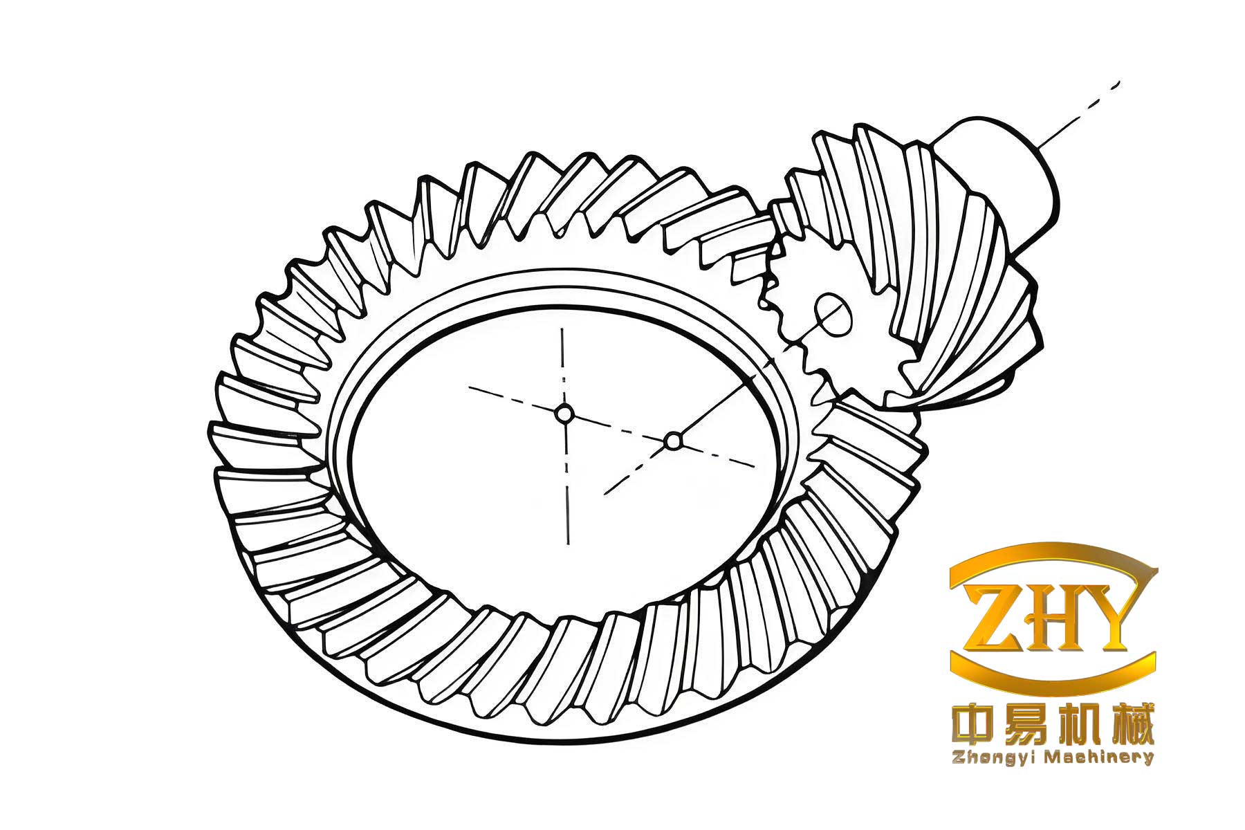
Hypoid gears are widely used in automotive drive systems, marine propulsion, and heavy mining equipment due to their smooth transmission, high load-carrying capacity, and low center of gravity. The traditional mechanical cradle-type machines, which are still the main equipment for machining hypoid gears in many domestic factories, suffer from complicated setup, low precision, and poor efficiency. The emergence of CNC cutting machines has brought new vitality to spiral bevel gear manufacturing, but due to the lack of a complete theoretical basis, most four-axis CNC machines are only used for cutting spiral bevel gears, not hypoid gears. To solve this problem, I have systematically studied the HFM (Formate gear, Modified-roll pinion) machining principle and successfully implemented it on a four-axis CNC cutting machine. This article presents my work on the mathematical models, local synthesis procedure, tooth contact analysis (TCA), coordinate transformations, and the experimental validation of the modified-roll method for hypoid gears.
## 1. Introduction and Motivation
The quality of hypoid gears is determined by the cutting machine, heat treatment process, and finishing method. The most advanced cutting machines are the Gleason Phoenix series, but they are too expensive for most domestic enterprises. Domestic four-axis CNC cutting machines, such as the YK2260X, are simple, rigid, and cost-effective. However, due to the lack of theoretical support, they could only machine spiral bevel gears. To expand their capability, I focused on the HFM method: the gear is cut by the formate process, while the pinion is generated by a modified-roll motion. This method avoids the disadvantages of the tilt method, such as discontinuous root fillets, and ensures a high production rate. The key challenge is to express the modified-roll motion correctly on a CNC machine, where the cradle rotation is replaced by linear X and Y axes.
## 2. Design of HFM Machining Parameters
### 2.1 Local Synthesis Methodology
The local synthesis method was introduced by Litvin to control the contact properties at the mean contact point. Unlike the traditional local conjugate approach, the local synthesis method allows the designer to preset:
– the position of the mean contact point,
– the length of the contact ellipse,
– the direction of the contact path,
– the first derivative of the transmission ratio at the mean contact point.
In my implementation, the gear is machined by the formate process, so its tooth surface is identical to the cutter cone surface. The pinion is generated by a cradle-type motion with a variable ratio of roll. The whole procedure is as follows:
1. Determine the gear cutting parameters.
2. Calculate the principal curvatures and directions of the gear tooth surface at the mean contact point.
3. Preset the desired contact characteristics and obtain the pinion principal curvatures and directions using surface point-contact theory.
4. Use the line-contact condition between the pinion surface and the imaginary generating gear to solve for the pinion machine settings.
### 2.2 Gear Formate Cutting Model
The gear cutting coordinate system is shown in Figure 2-3 of the original study. The cutter coordinate system is \(S_e\), the machine coordinate system is \(S_m\), and the gear coordinate system is \(S_2\). The gear tooth surface is expressed as:
\[
\mathbf{r}_2(u_G,\theta_G) = [M_{2m}][M_{mg}][M_{ge}] \mathbf{r}_e(u_G,\theta_G)
\]
where the cutter surface is a cone:
\[
\mathbf{r}_e(u_G,\theta_G) =
\begin{bmatrix}
r_{c2} – u_G \cos\alpha_2 \cos\theta_G \\
– (r_{c2} – u_G \cos\alpha_2) \sin\theta_G \\
-u_G \sin\alpha_2 \\
1
\end{bmatrix}
\]
The unit normal vector is:
\[
\mathbf{n}_e(\theta_G) =
\begin{bmatrix}
\sin\alpha_2 \\
-\cos\alpha_2 \sin\theta_G \\
-\cos\alpha_2 \cos\theta_G
\end{bmatrix}
\]
The gear is formate-cut, meaning that the cradle is fixed during machining. Thus, the gear tooth surface is exactly the same as the cutter surface. The principal directions on the conical cutter surface are:
\[
\mathbf{e}_I^e = \begin{bmatrix} -\sin\theta_G \\ \cos\theta_G \\ 0 \end{bmatrix}, \quad
\mathbf{e}_{II}^e = \begin{bmatrix} \cos\alpha_2 \cos\theta_G \\ -\cos\alpha_2 \sin\theta_G \\ -\sin\alpha_2 \end{bmatrix}
\]
and the corresponding principal curvatures are:
\[
k_I^G = \frac{\cos\alpha_2}{r_{c2}-u_G\cos\alpha_2}, \quad k_{II}^G = 0
\]
After the coordinate transformation, the principal directions are expressed in the global coordinate system \(S_h\) at the mean contact point.
### 2.3 Mean Contact Point Specification
The mean contact point is usually chosen near the center of the tooth flank. For the gear, the point is defined by the coordinates \(XL\) and \(RL\) in the axial and radial directions. Solving the nonlinear equations gives the cutter surface parameters \(u_G^*\) and \(\theta_G^*\). Then, the gear tooth surface position and normal at this point are obtained.
### 2.4 Local Synthesis for the Pinion
At the mean contact point, the gear and the pinion tooth surfaces are in point contact. The following parameters must be specified before solving for the pinion characteristics:
– Transmission ratio \(m_{21} = N_1/N_2\).
– First derivative of the transmission ratio at the mean contact point: \(m_{21}’\), which is chosen negative to obtain a parabolic transmission error function with a positive apex.
– The contact ellipse major semi-axis length \(b\). A positive value is used for the convex side of the pinion, and a negative value for the concave side.
– The angle \(\eta_2\) between the contact path tangent and the first principal direction on the gear surface.
Using the theory of two mating surfaces in point contact, the following fundamental equations are solved to obtain the pinion principal directions and curvatures:
\[
\mathbf{v}_{12} \cdot \mathbf{n} = 0
\]
\[
\mathbf{v}_{12} = \boldsymbol{\omega}^{(1)} \times \mathbf{r}_h – \boldsymbol{\omega}^{(2)} \times \mathbf{r}_h
\]
\[
m_{21}’ = f(\eta_2, b, k_I^{(1)}, k_{II}^{(1)})
\]
The result is the set of pinion principal curvatures \(k_I^{(1)}, k_{II}^{(1)}\) and principal directions \(\mathbf{e}_I^{(1)}, \mathbf{e}_{II}^{(1)}\) in the fixed coordinate system.
### 2.5 Pinion Generating Model and Line-Contact Equations
The pinion is generated by an imaginary crown gear. The pinion tooth surface and the generating surface are in line contact. In the coordinate system \(S_c\), the relative velocity between the cutting tool and the pinion is:
\[
\mathbf{v}^{(f1)} = \boldsymbol{\omega}^{(f)} \times \mathbf{r} – \boldsymbol{\omega}^{(1)} \times \mathbf{r} + \mathbf{O}_f^{(f)} – \mathbf{O}_1^{(1)}
\]
The line-contact condition requires that the relative velocity vector lies in the common tangent plane, leading to:
\[
\mathbf{n} \cdot \mathbf{v}^{(f1)} = 0
\]
After expressing all vectors in the coordinate system \(S_c\), I derived the following set of equations:
\[
b_{11} b_{22} – b_{12}^2 = 0
\]
\[
b_{11} b_{23} – b_{12} b_{13} = 0
\]
\[
b_{12} b_{33} – b_{13} b_{23} = 0
\]
where the coefficients \(b_{ij}\) involve the principal curvatures of the pinion and the generating tool at the contact point. Solving these equations yields the pinion machine settings:
– Radial cutter position \(S_1\),
– Angular cutter position \(q_1\),
– Vertical offset \(E_1\),
– Horizontal wheel position \(X_1\),
– Sliding base \(X_{B1}\),
– Ratio of roll \(R_{ap}\) or the machine root angle \(\gamma_1\).
The cutting tool for the pinion has a cone angle \(\alpha_1\), and its principal curvatures are:
\[
k_I^{(f)} = \frac{\cos\alpha_1}{r_{c1} + u_q \sin\alpha_1}, \quad k_{II}^{(f)} = 0
\]
where \(r_{c1}\) is the pinion cutter point radius and \(u_q\) is the surface parameter.
### 2.6 Modified-Roll Polynomial
For the modified-roll process, the relationship between the workpiece rotation angle \(\phi_1\) and the cradle rotation angle \(\phi_f\) is not linear. In my work, I used a fifth-order Taylor series representation:
\[
\phi_1(\phi_f) = R_{ap} \phi_f – C_2 \phi_f^2 – D_3 \phi_f^3 – E_4 \phi_f^4 – F_5 \phi_f^5
\]
where \(R_{ap}\) is the basic ratio of roll at the mean contact point. The coefficients \(C_2, D_3, E_4, F_5\) are related to the higher-order derivatives of the roll ratio. In practice, the second-order coefficient \(C_2\) is usually called the “second-order modified-roll coefficient” and the third-order coefficient \(D_3\) is the “third-order modified-roll coefficient.” These coefficients are expressed as:
\[
C_2 = -\frac{1}{2} \left.\frac{d^2\phi_1}{d\phi_f^2}\right|_{\phi_f=0}
\]
\[
D_3 = -\frac{1}{6} \left.\frac{d^3\phi_1}{d\phi_f^3}\right|_{\phi_f=0}
\]
The coefficients have a strong influence on the tooth flank geometry and the transmission error curve, as shown in Chapter 3.
## 3. Tooth Contact Analysis
### 3.1 TCA Model
The TCA program simulates the meshing of the gear and pinion in the coordinate system \(S_h\). The gear tooth surface is already known from the formate process. The pinion tooth surface is generated according to the modified-roll motion. The meshing equations are:
\[
\mathbf{r}_h^{(1)}(\theta_q, \phi_q, \beta_1) = \mathbf{r}_h^{(2)}(u_G, \theta_G, \beta_2)
\]
\[
\mathbf{n}_h^{(1)}(\theta_q, \phi_q, \beta_1) = \mathbf{n}_h^{(2)}(u_G, \theta_G, \beta_2)
\]
where \(\beta_1\) and \(\beta_2\) are the rotation angles of the pinion and the gear during meshing, respectively. Since \(\mathbf{n}_h\) is a unit normal vector, the second vector equation gives only two independent scalar equations. Thus, five independent scalar equations remain for six unknowns. By fixing \(\beta_2\), the system can be solved for the five remaining unknowns. Repeating this process for a sequence of \(\beta_2\) values gives the contact path and the transmission error.
The transmission error is defined as:
\[
\delta(\beta_1) = \beta_2 – \beta_2^{(0)} – \frac{N_1}{N_2} (\beta_1 – \beta_1^{(0)})
\]
where \(\beta_1^{(0)}, \beta_2^{(0)}\) are the angles at the mean contact point. A good gear set should have a parabolic transmission error curve with a positive value at the center, so that the gear lags behind the theoretical rotation. This helps absorb shocks and reduces sensitivity to assembly errors.
### 3.2 V/H Test Simulation
The V/H test is a standard method for evaluating the sensitivity of the contact pattern to changes in the mounting distance. In my TCA program, I simulated the V/H test by introducing a vertical offset \(V\) and a horizontal offset \(H\) in the meshing model, as shown in Figure 3-2. The new coordinates become:
\[
\mathbf{r}_h^{(2)} = \mathbf{r}_h^{(2)} + \begin{bmatrix} 0 \\ V \\ 0 \end{bmatrix}
\]
\[
\mathbf{r}_h^{(1)} = \mathbf{r}_h^{(1)} + \begin{bmatrix} 0 \\ 0 \\ H \end{bmatrix}
\]
The contact point at the middle of the gear face is prescribed by solving the six equations with the additional condition that the instantaneous transmission ratio is equal to the theoretical ratio. This determines the required V/H values for the target point.
### 3.3 Influence of the Second-Order Modified-Roll Coefficient
Using my TCA program, I analyzed the effect of changing the second-order coefficient \(C_2\) on the pinion concave and convex flanks. The gear set employed for the analysis has \(N_1 = 6\), \(N_2 = 37\), and a module of 11.732 mm. The basic pinion settings are listed in Table 3-3. I will show the main results.
The following table summarizes the effect of \(C_2\) on the pinion concave flank:
| Parameter | Base value | Increased \(C_2\) by 0.02 | Effect |
|—|—|—|—|
| Contact path | nearly straight | nearly straight | no visible change |
| Transmission error intersection | 28 (point) | 65 | parabolic shape remains, amplitude increases |
| Transmission error bottom | about 50 | about 100 | larger amplitude improves alignment |
| Tooth curvature | original | lengthwise curvature becomes smaller | spiral angle decreases |
| Flank twist | original | twist changes significantly | pressure angle changes differently at toe and heel |
The tooth surface deviation plot (Figure 3-5 in the original) showed that the deviation is distributed along the whole flank, with a U-shaped pattern in the lengthwise direction.
For the pinion convex flank, the influence was also analyzed. The base second-order coefficient is \(-0.1755\). After increasing it by 0.02, the main observations are:
| Parameter | Base value | Increased \(C_2\) by 0.02 |
|—|—|—|
| Contact path | almost straight | almost straight |
| Transmission error intersection | 30 | 10 |
| Transmission error bottom | 45 | 15 |
| Lengthwise curvature | original | becomes larger |
| Flank twist | original | changes sign in the nonlinear region |
The second-order coefficient dominates the second-order deviation of the flank, which directly affects the lengthwise curvature and the pressure angle at the toe and heel.
### 3.4 Influence of the Third-Order Modified-Roll Coefficient
The third-order coefficient \(D_3\) was also studied. For the pinion concave side, \(D_3\) was changed from \(-0.13\) to \(-0.08\). The results are shown in the following table:
| Parameter | Base value | Increased \(D_3\) by 0.05 |
|—|—|—|
| Contact path | almost straight | almost straight |
| Transmission error intersection | no obvious change | no obvious change |
| Transmission error bottom | about 50 | about 70 |
| Spiral angle | original | becomes smaller |
| Pressure angle | original | becomes smaller along the flank from toe to heel |
For the pinion convex side, the base \(D_3 = 0\). After increasing \(D_3\) to \(0.05\), the influence is similar to that on the concave side: the spiral angle becomes smaller and the pressure angle is reduced. The main difference is that the third-order coefficient changes the curvature variation along the flank, leading to a non-linear deviation in both lengthwise and profile directions.
The above analysis shows that the second-order coefficient \(C_2\) is the main tool for adjusting the lengthwise curvature and the transmission error amplitude, while the third-order coefficient \(D_3\) can be used to fine-tune the tooth surface topology without significantly changing the transmission error intersection. By properly selecting \(C_2\) and \(D_3\), one can obtain an excellent contact pattern and a smooth parabolic transmission error curve.
## 4. CNC Cutting Machine Motion
### 4.1 Machine Tool Structure
The four-axis CNC cutting machine YK2260X has four controlled axes:
– \(X\): horizontal linear axis,
– \(Y\): vertical linear axis,
– \(Z\): feed axis (used to control the depth of cut),
– \(A\): workpiece spindle rotation axis.
During generation, the \(X\), \(Y\), and \(A\) axes are simultaneously interpolated. The \(X\) and \(Y\) axes simulate the cradle rotation. The tool spindle rotates independently. The \(Z\) axis is only used for feeding and retracting.
### 4.2 Coordinate Transformation
The first task is to map the theoretical machine settings to the CNC coordinate system. The theoretical pinion coordinate system \(S_6\) has its origin at the center of the cradle. The cutter center \(O_c\) is located at a distance \(S_1\) from \(O_6\), with an angular position \(q_1\). After transforming to the workpiece coordinate system, the cutter center coordinates are:
\[
C = \frac{H_1 – X_1 \cos\delta_f}{\cos\delta_f}
\]
\[
D = V_1 – E_1
\]
where \(H_1\) and \(V_1\) are the horizontal and vertical components of the radial cutter position:
\[
H_1 = S_1 \cos q_1, \quad V_1 = S_1 \sin q_1
\]
Here, \(\delta_f\) is the machine root angle of the pinion.
The CNC machine has a fixed pivot point \(O_4\) and a zero reference point \(O_3\). The distance between \(O_3\) and \(O_4\) is a machine constant \(L\). The workpiece is mounted on a fixture with length \(L_1\) and the gear mounting distance \(L_2\). Thus, the cutter center in the machine base coordinate system \(S_0\) is:
\[
C_0 = M + (H_1 – X_1 \cos\delta_f – L_1 – L_2 – L) \cos\delta_f
\]
\[
D_0 = V_1 – E_1 + N
\]
where \(M\) and \(N\) are the coordinates of the rotary table center in the machine coordinate system. These values are known from the machine tool design.
### 4.3 Cutting Start and End Positions
In the CNC machine, the cutter center moves along a circular arc that simulates the cradle rotation. The virtual cradle center is \(O_6\), and the radial cutter position is \(S_1\). The total generation angle (cradle angle) is \(\theta\). The cutting starts at an angle \(q_1 + \theta/2\) and ends at \(q_1 – \theta/2\), as shown in Figure 4-6. In the temporary workpiece coordinate system \(S_8\), the starting point is:
\[
X_{s1} = S_1 \cos(q_1 + \theta/2)
\]
\[
Y_{s1} = S_1 \sin(q_1 + \theta/2)
\]
and the ending point is:
\[
X_{s2} = S_1 \cos(q_1 – \theta/2)
\]
\[
Y_{s2} = S_1 \sin(q_1 – \theta/2)
\]
During the cutting process, the instantaneous position is:
\[
X_8 = S_1 \cos q
\]
\[
Y_8 = S_1 \sin q
\]
where \(q\) varies linearly from \(q_1 + \theta/2\) to \(q_1 – \theta/2\).
The workpiece spindle angle \(A\) is given by the modified-roll polynomial. For the CNC interpolation, I used the following expression:
\[
A = A_0 + R_{ap} (q – q_0) – C_2 (q – q_0)^2 – D_3 (q – q_0)^3
\]
where \(A_0\) is the workpiece angle at the mean contact point, and \(q_0 = q_1\) is the angular position at the mean contact point.
### 4.4 Numerical Control Program Structure
The CNC program was written in Siemens 802D format. The main steps are:
1. Home the machine and set the workpiece coordinate system origin at the tool-setting position.
2. Move \(X\) and \(Y\) to the starting position \(X_{s1}, Y_{s1}\) with \(A\) at the corresponding value.
3. Feed the \(Z\) axis to the proper depth.
4. Execute a loop of interpolation steps. At each step, \(q\) is incremented by a small angle \(\Delta q\). The corresponding \(X\), \(Y\), and \(A\) values are computed and commanded as a linear interpolation segment.
5. After the total number of steps is reached, the \(Z\) axis is retracted.
6. The workpiece is indexed to the next tooth gap.
7. The process repeats until all teeth are cut.
The step size \(\Delta q\) was set to \(0.25^\circ\) in the initial experiments, and later reduced to \(0.125^\circ\) to improve the surface finish. The interpolation formula is:
\[
q_{k+1} = q_k + \Delta q
\]
\[
X_k = S_1 \cos q_k, \quad Y_k = S_1 \sin q_k
\]
\[
A_k = A_0 + R_{ap}(q_k – q_0) – C_2(q_k – q_0)^2 – D_3(q_k – q_0)^3
\]
## 5. Cutting Experiment
### 5.1 Experimental Setup
The experiment was performed on a YK2260X four-axis CNC hypoid gear cutting machine, controlled by a Siemens 802D CNC system. The machine is equipped with an 11 kW inverter-driven spindle motor. The workpiece is automatically clamped, and the fixture is compatible with the Y2280 mechanical machine.
The gear set used for the experiment has the following parameters:
| Parameter | Pinion | Gear |
|—|—|—|
| Number of teeth | 6 | 41 |
| Module (mm) | 10.588 | 10.588 |
| Face width (mm) | 67.2 | 62 |
| Offset (mm) | 35 | – |
| Shaft angle (deg) | 90 | 90 |
| Outer cone distance (mm) | 213.192 | 220.678 |
| Addendum (mm) | 13.603 | 1.644 |
| Dedendum (mm) | 3.788 | 15.487 |
| Whole depth (mm) | 17.39 | 17.15 |
| Pitch angle (deg) | 10.22 | 79.6 |
| Root angle (deg) | 9.82 | 76.33 |
| Face angle (deg) | 13.43 | 80 |
| Spiral direction | Left hand | Right hand |
### 5.2 Pinion Cutting Parameters
The pinion was cut by the modified-roll process. The final machining parameters after the V/H correction are listed below:
| Parameter | Concave side | Convex side |
|—|—|—|
| Cutter radius (mm) | 143.345 | 159.25 |
| Cutter blade angle (deg) | 20.133 | 24.5 |
| Machine root angle (deg) | 9.82 | 9.82 |
| Radial cutter position (mm) | 176.53 | 152.9 |
| Angular cutter position (deg) | -62.13335 | -63.0833 |
| Vertical offset (mm) | 49.86 | 25.31 |
| Horizontal wheel position (mm) | 7.43 | -6.7 |
| Sliding base (mm) | -4.72 | -2.04 |
| Ratio of roll | 7.703375 | 6.377562 |
| Second-order coefficient | 0.209965 | -0.176999 |
| Third-order coefficient | 0 | 0.08 |
The gear was formate-cut with the following parameters:
| Parameter | Value |
|—|—|
| Radial cutter position (mm) | 162.2794 |
| Angular cutter position (deg) | 50.8 |
| Horizontal wheel position (mm) | -0.628 |
| Machine root angle (deg) | 76.3333 |
| Cutter radius (mm) | 152.4 |
| Blade offset (mm) | 5.33 |
| Outside blade angle (deg) | 22.5 |
| Inside blade angle (deg) | 22.5 |
### 5.3 Contact Pattern Correction and Results
After the first cutting, the roll test showed that the working side (convex side of the gear / concave side of the pinion) had a contact pattern near the toe and slightly below the center, with a diffuse middle area. The non-working side had a long contact pattern near the root and shifted toward the heel. According to the conventional correction rules:
– To move the contact toward the toe on the non-working side, the radial cutter position should be decreased.
– To move the contact toward the top, the ratio of roll should be increased.
The first correction for the non-working side was:
\[
\Delta S_1 = -0.1 \ \text{mm}, \quad \Delta R_{ap} = +0.015
\]
After machining, the contact pattern moved to the proper position but was still too wide and too long. To narrow the contact, the vertical offset was increased by 6 mm, which required a corresponding increase in the radial cutter position, horizontal wheel position, and ratio of roll. The exact values were determined using the local synthesis sensitivity equations:
\[
\Delta S_1 = 4.7497 \ \text{mm}, \quad \Delta X_1 = 0.95 \ \text{mm}, \quad \Delta R_{ap} = 0.184
\]
In addition, the cutter radius was reduced by 2.4 mm to shorten the contact length. After applying these corrections, the non-working side showed an ideal contact pattern: located in the central area of the flank, with no edge contact.
The working side was corrected by reducing the radial cutter position by 0.42 mm and the horizontal wheel position by 0.6 mm. The final roll test showed a good contact pattern with a length of about one-third of the face width and a height of about one-half of the tooth depth. No diagonal contact or edge loading was observed. The noise was acceptable for a spiral bevel gear set.
### 5.4 Discussion on Interpolation Step Size
The modified-roll motion on a CNC machine is realized by small linear interpolation segments. The approximation error is proportional to the square of the step angle \(\Delta q\). For a step size of \(0.25^\circ\), the machined surface was already smooth. By reducing the step to \(0.125^\circ\), the tooth surface roughness was further improved without increasing the machining time substantially. The final experiment used a step size of \(0.125^\circ\). The successful results prove that the derived motion equations are correct and that the four-axis CNC machine can be used for manufacturing high-quality hypoid gears.
## 6. Conclusions and Outlook
In this work, I have systematically studied the HFM method for manufacturing hypoid gears on a four-axis CNC cutting machine. The main conclusions are as follows:
1. The local synthesis method was successfully applied to design the pinion machining parameters for the modified-roll process. The gear is formate-cut, and the pinion is generated with a variable ratio of roll. The derived mathematical models give the cutter geometry and all machine settings.
2. The modified-roll motion can be accurately represented by a fifth-order Taylor polynomial. The second-order coefficient \(C_2\) and the third-order coefficient \(D_3\) have significant effects on the tooth surface topology. My TCA analysis showed that \(C_2\) primarily controls the lengthwise curvature and the transmission error amplitude, while \(D_3\) adjusts the flank twist and the nonlinear variation of the spiral angle and pressure angle.
3. The TCA program, combined with V/H simulation, provides a powerful tool for optimizing the cutting parameters without performing multiple trial cuts. It allows the designer to predict contact patterns and transmission error curves with high accuracy.
4. The coordinate transformation between the theoretical cradle-type machine and the four-axis CNC machine was established. The tool-setting position, the cutting start and end positions, and the instantaneous positions of the \(X\), \(Y\), and \(A\) axes were explicitly derived. The numerical control program was written in Siemens 802D format.
5. A cutting experiment was carried out on a YK2260X machine for a gear set with 6 pinion teeth and 41 gear teeth. After a few correction loops, the contact pattern was excellent, and the noise level was acceptable. This validates the feasibility of manufacturing hypoid gears on domestic four-axis CNC cutting machines.
Future work should focus on the development of an automatic correction method based on tooth surface measurement. The current correction approach still relies on the traditional proportional correction rules, which are empirical. Furthermore, the software needs to be improved with a user-friendly interface and should incorporate constraints such as root undercut, tool interference, and machine travel limits. Another interesting direction is to use the high flexibility of CNC machines to produce tooth surfaces with predetermined higher-order transmission error curves, which can further improve the dynamic behavior of hypoid gear drives.
The successful implementation of the modified-roll method on a four-axis CNC machine is an important step toward the full digitalization of hypoid gear manufacturing. It provides a cost-effective solution for domestic enterprises that cannot afford six-axis free-form machines, while greatly expanding the capability of existing four-axis CNC equipment. The results of this research offer a solid theoretical foundation for the development of dedicated hypoid gear cutting software and will contribute to the advancement of gear manufacturing technology in China.