
In modern mechanical transmission systems, spur gears are among the most widely used components. They transmit power and torque through tooth engagement, and their reliability directly affects the overall system performance. Tooth surface wear is one of the most common failure modes in spur gears. It changes the tooth profile, increases vibration and noise, reduces transmission efficiency, and eventually leads to system breakdown. Therefore, understanding the wear evolution mechanism and developing a quantitative evaluation method for spur gears is of great engineering significance. In this thesis, I focus on the modeling of tooth surface wear for spur gears and the quantitative assessment based on vibration signal analysis. I first establish a line-contact mixed elastohydrodynamic lubrication (EHL) wear model, then investigate the effect of wear on time-varying meshing stiffness and dynamic characteristics, and finally propose a vibration-based quantitative evaluation method for tooth surface wear of spur gears.
1. Introduction
Gear transmission systems are found in vehicles, aircraft engines, marine propulsion systems, agricultural machinery, and many other industrial applications. Compared with belt drives or hydraulic transmissions, gear drives offer higher efficiency, more accurate transmission ratios, and better durability. However, gears operate under harsh conditions with high contact pressure, sliding, and repeated loading, which makes wear inevitable. Tooth surface wear in spur gears is a progressive phenomenon. It not only alters the geometric profile of the teeth but also affects the contact stress distribution, lubricating condition, and dynamic response. The consequences of wear include increased vibration, higher noise, reduced fatigue life, and even catastrophic failure.
Research on gear wear can be traced back to the classical Archard wear law. Archard proposed that the wear volume is proportional to the normal load and sliding distance and inversely proportional to the material hardness. Based on this law, many scholars have developed numerical models to predict the wear depth distribution on gear tooth surfaces. Flodin and Andersson introduced a quasi-static wear model for spur gears by discretizing the tooth profile and updating the geometry after a certain number of load cycles. Wu and Cheng incorporated mixed lubrication effects into the wear calculation. Subsequent studies have considered more factors such as tooth profile modifications, misalignment, surface roughness, and lubricant properties.
However, most existing wear models for spur gears ignore the coupling between dynamic load and wear. In reality, as wear progresses, the dynamic behavior of the gear pair changes, which in turn influences the wear rate. Moreover, many studies only consider uniform wear along the tooth width, which is not sufficient for non-uniform wear patterns in spur gears. There is a need for a comprehensive model that integrates contact mechanics, mixed lubrication, flash temperature, and dynamic loading to predict the wear depth distribution accurately.
In this thesis, I take a spur gear pair with a contact ratio between 1 and 2 as the research object. I first derive a line-contact mixed EHL wear model based on the Archard equation. The model includes the calculation of tooth contact parameters, sliding distance, lubricant film thickness, asperity contact ratio, and flash temperature. I then calculate the time-varying meshing stiffness of worn spur gears using the energy method and verify the results by finite element analysis. I also establish a torsional vibration model to study the dynamic response of the gear pair with tooth surface wear. Finally, I analyze the evolution of vibration signal characteristic parameters and propose a quantitative method for estimating the wear depth from vibration signals.
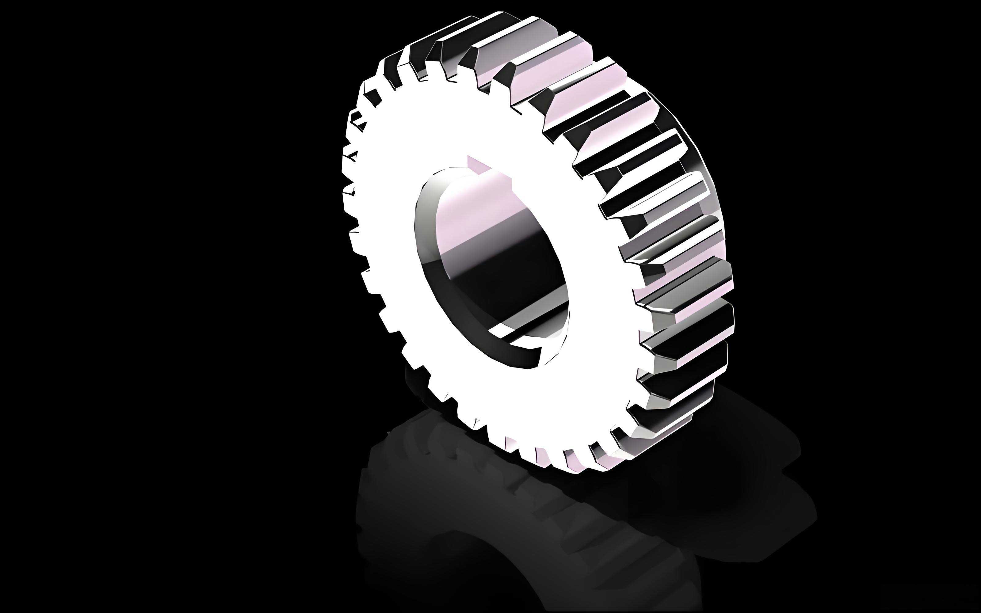
2. Tooth Surface Wear Calculation Method for Spur Gears
2.1 Gear Meshing Geometry and Contact Parameters
The spur gear pair considered in this study has the following basic parameters: module \(m = 2\,\text{mm}\), number of teeth on the pinion \(z_1 = 18\), number of teeth on the gear \(z_2 = 27\), pressure angle \(\alpha = 20^\circ\), face width \(B = 30\,\text{mm}\), addendum coefficient \(h_a^* = 1\), and clearance coefficient \(c^* = 0.25\). The standard center distance is \(A = m(z_1+z_2)/2 = 45\,\text{mm}\). The pitch circle radii are \(r_1 = m z_1 / 2 = 18\,\text{mm}\) and \(r_2 = m z_2 / 2 = 27\,\text{mm}\). The base circle radii are \(r_{b1} = r_1 \cos\alpha\) and \(r_{b2} = r_2 \cos\alpha\).
For a spur gear pair, the actual line of contact starts at the intersection of the pinion base circle and the gear addendum circle (point \(B_1\)) and ends at the intersection of the pinion addendum circle and the gear base circle (point \(B_2\)). The length of the line of action is given by
$$B_1B_2 = \sqrt{r_{a1}^2 – r_{b1}^2} + \sqrt{r_{a2}^2 – r_{b2}^2} – (r_1 + r_2)\sin\alpha.$$
The contact ratio \(\varepsilon\) is defined as
$$\varepsilon = \frac{B_1B_2}{p_b},$$
where \(p_b = \pi m \cos\alpha\) is the base pitch. The contact ratio for the studied gear pair is between 1 and 2, so there are alternating zones of single-tooth and double-tooth engagement.
At a meshing point \(k\), the radii of curvature of the pinion and gear are computed as \(R_{1k} = r_{b1}\tan\alpha_{1k}\) and \(R_{2k} = r_{b2}\tan\alpha_{2k}\), where \(\alpha_{1k}\) and \(\alpha_{2k}\) are the pressure angles at that point. The equivalent radius of curvature is
$$\frac{1}{R_k} = \frac{1}{R_{1k}} + \frac{1}{R_{2k}}.$$
Following the Hertz contact theory, the half-width of the contact zone is
$$b_H = \sqrt{\frac{8 W R_k}{\pi E_z}},$$
where \(W\) is the normal load per unit face width, and \(E_z\) is the equivalent elastic modulus defined by
$$\frac{1}{E_z} = \frac{1-\delta_1^2}{E_1} + \frac{1-\delta_2^2}{E_2}.$$
The maximum Hertz contact pressure is \(p_{\max} = 2W/(\pi b_H)\), and the average pressure is \(p_{avg} = 4p_{\max}/\pi\).
2.2 Load Sharing in Double-Tooth Engagement
Since the contact ratio is between 1 and 2, the load is shared by either one pair or two pairs of teeth. In the single-tooth contact zone, the load per unit width is \(W = F_n / B\), where \(F_n\) is the normal force. In the double-tooth contact zone, the load distribution depends on the stiffness of the two tooth pairs and the geometric gap caused by wear. Let \(h_{w1}(y)\) and \(h_{w2}(y)\) denote the wear depths on the pinion and gear at a position \(y\) relative to the pitch point. The additional gap due to wear can be expressed in different ways depending on whether the contact is in the incoming or outgoing double-tooth zone. Then the unit load on the first pair is
$$W_1 = \frac{M_1 (F_n/B \pm |\Delta| M_2)}{M_1 + M_2},$$
and similarly for the second pair. Here \(M_1\) and \(M_2\) are the time-varying meshing stiffness values of the two tooth pairs, and \(\Delta\) is the gap caused by wear. A more detailed description can be found in the literature.
2.3 Sliding Velocity and Sliding Distance
The tangential velocities of the pinion and gear at a meshing point are \(v_1 = \omega_1 R_1\) and \(v_2 = \omega_2 R_2\), respectively. The sliding velocity is
$$v_s = |v_1 – v_2|,$$
and the entraining velocity is
$$v_e = \frac{v_1 + v_2}{2}.$$
During one meshing cycle, the sliding distance on the pinion and gear can be approximated by
$$L_1 = 2 b_H \left|1 – \frac{v_2}{v_1}\right|, \quad L_2 = 2 b_H \left|1 – \frac{v_1}{v_2}\right|.$$
At the pitch point, the sliding velocity is zero because the two tangential velocities are equal. Consequently, the sliding distance is minimal there. The sliding distance reaches its maximum near the root of the pinion and the tip of the gear, which explains why the wear depth is largest at those locations.
2.4 Line-Contact Mixed Elastohydrodynamic Lubrication Model
In practice, spur gears often operate in a mixed lubrication regime where the load is carried partly by the lubricant film and partly by the asperities of the rough surfaces. To accurately predict wear, I employ a line-contact mixed EHL model. The model combines the Reynolds equation, film thickness equation, viscosity-pressure equation, density-pressure equation, and load balance equation with the Greenwood-Williamson type statistical asperity contact model.
The modified Reynolds equation for rough line contacts is written as
$$\frac{\partial}{\partial x}\left(\phi_x \frac{\rho h^3}{\eta}\frac{\partial p}{\partial x}\right) = 12 v_e \frac{\partial (\rho \bar{h}_T)}{\partial x},$$
where \(\phi_x\) is the pressure flow factor, \(h\) is the nominal film thickness, \(\bar{h}_T\) is the average gap, \(\rho\) and \(\eta\) are the density and viscosity of the lubricant, and \(p\) is the hydrodynamic pressure. The total pressure is composed of the hydrodynamic contribution and the asperity contact pressure:
$$p_{total} = p_h + p_a.$$
The film thickness equation includes the elastic deformation term:
$$h(x) = h_0 + \frac{x^2}{2R} – \frac{2}{\pi E_z} \int_{x_i}^{x_o} p(s) \ln(s-x)^2 \, ds.$$
The viscosity-pressure relationship used in this thesis is the Barus-like equation with temperature correction:
$$\eta = \eta_0 \exp\left\{ \ln(\eta_0/10^{-9}) \left[ \left(1 + \frac{p}{1.98\times 10^8} \right)^{0.68} – 1 \right] \right\}.$$
The density-pressure relationship is
$$\rho = \rho_0 \left(1 + \frac{0.6 p}{1 + 1.7 p}\right).$$
To solve the mixed EHL problem, a numerical iterative scheme is adopted. In this thesis, I use the empirical regression formulas proposed by Masjedi and Khonsari for the minimum film thickness and the asperity contact ratio. The dimensionless minimum film thickness is
$$H_{\min} = \frac{h_{\min}}{R} = 1.652 W^{-0.077} U^{0.716} G^{0.695} \left(1 + 0.026 \frac{\bar{\sigma}}{R}\right)^{-0.312},$$
where \(W\), \(U\), and \(G\) are the dimensionless load, speed, and material parameters, and \(\bar{\sigma}\) is the dimensionless surface roughness. The asperity contact ratio \(L_a\) (the ratio of asperity contact load to total load) is
$$L_a = 0.005 W^{-0.408} U^{-0.088} G^{-0.103} V^{0.485} \ln\left(1 + 4470 \bar{\sigma}\right),$$
where \(V\) is the dimensionless hardness. With \(L_a\), the hydrodynamic pressure and asperity pressure can be separated as
$$p_h = p_{total} (1 – L_a/100), \quad p_a = p_{total} L_a/100.$$
The film thickness ratio \(\Lambda = h_{\min}/\sigma\) indicates the lubrication regime. In the present work, \(\Lambda\) lies typically between 1 and 2.5, confirming that the gears operate in the mixed lubrication regime.
2.5 Flash Temperature Calculation
To account for thermal effects, I calculate the flash temperature rise at the contacting surfaces. According to Tian and Kennedy’s model, the flash temperature is
$$\Delta T = \frac{2 b_H q}{\sqrt{\pi} \left( \frac{K_1}{\sqrt{k_1 v_1}} + \frac{K_2}{\sqrt{k_2 v_2}} \right)},$$
where \(q\) is the heat flux generated at the contact. The heat flux consists of two parts: heat generated by asperity friction and heat generated by shear of the lubricant film. The total heat flux is expressed as
$$q = f_c v_s p_a + \Lambda_{\lim} v_s p_h,$$
where \(f_c\) is the dry friction coefficient and \(\Lambda_{\lim}\) is the limiting shear stress coefficient. The bulk temperature is set to \(T_0 = 315\,\text{K}\), and the instantaneous contact temperature is \(T = T_0 + \Delta T\). Both viscosity and density are updated using this temperature.
2.6 Wear Model and Numerical Implementation
The wear depth at a point is calculated using the Archard wear law in its local form:
$$\frac{dh}{ds} = \frac{k p}{H},$$
where \(k\) is the dimensionless wear coefficient, \(p\) is the local contact pressure, \(H\) is the material hardness, and \(ds\) is the sliding distance. In the mixed lubrication regime, only the asperity contact pressure contributes to wear. Therefore, the wear depth increment after a small number of cycles is
$$dh = k \left(\frac{L_a}{100}\right) p_{total} \frac{L}{H} \psi,$$
where \(L\) is the sliding distance and \(\psi\) is an oil film deficiency coefficient given by
$$\psi = 1 – \exp\left[ -\frac{E_a}{R_g T}\right] \exp\left[ -\frac{X}{v_s t_0}\right].$$
Here \(X\) is the molecular diameter of the lubricant, \(t_0\) is the molecular vibration time, \(E_a\) is the adsorption heat, and \(R_g\) is the gas constant. In this thesis, I set \(X = 3\times10^{-10}\,\text{m}\), \(t_0 = 3\times10^{-12}\,\text{s}\), and \(E_a = 4.9\times10^4\,\text{J/mol}\).
The wear depth is integrated over the tooth flank by discretizing the profile into small segments. After each block of cycles, if the total wear depth changes by more than 1 μm, the tooth profile is updated. The new radius of curvature becomes
$$R_{new} = R_{old} – h_w.$$
Then all contact calculations are repeated. The wear computation flow is summarized as follows:
- Compute meshing geometry and load distribution.
- Solve the mixed EHL model to obtain film thickness and asperity contact ratio.
- Calculate flash temperature and oil film deficiency coefficient.
- Compute wear depth increment for the current cycle block.
- Update tooth profile if necessary.
- Repeat until the desired number of cycles is reached.
2.7 Numerical Results and Discussion
Table 1 lists the operating conditions used in the baseline simulation.
| Parameter | Value |
|---|---|
| Input speed \(n_1\) (r/min) | 2000 |
| Load torque \(T_{N2}\) (N·m) | 300 |
| Lubricant viscosity \(\eta_0\) (Pa·s) | 0.35 |
| Pressure-viscosity coefficient \(\alpha_y\) (m²/N) | 2.5×10⁻⁸ |
| Limiting shear stress coefficient \(\Lambda_{\lim}\) | 0.0910 |
| Surface roughness \(\sigma\) (μm) | 0.5 |
| Wear coefficient \(k\) | 5×10⁻⁴ |
The simulation is run for 1×10⁶ cycles. The wear depth distributions along the pinion and gear tooth profiles are analyzed. Figure 1 shows the typical wear distribution shape: the wear depth decreases from the tooth root to the pitch point and then increases toward the tooth tip. The minimum wear depth occurs at the pitch point, while the maximum wear depth occurs at the pinion root and at the gear tip. The pinion wear is generally larger than the gear wear because the pinion has fewer teeth and rotates more times for the same number of gear cycles.
A notable feature is the sudden change in wear depth at the transition between single-tooth and double-tooth engagement zones. This is caused by the abrupt change in load sharing and sliding distance. In the double-tooth zone, the load per tooth is lower, but the sliding distance may be larger near the extremes. The combination of these effects produces the observed discontinuity.
2.7.1 Effect of Number of Cycles
As the number of wear cycles increases, the wear depth at every point increases. The wear rate is not constant because the tooth profile changes and the load distribution is altered. The pinion root point shows the highest wear rate, which means that early wear is most severe at the root. After 1.5×10⁶ cycles, the pinion root wear is about 1.2 μm.
2.7.2 Effect of Input Speed
Three input speeds are considered: 1000, 2000, and 3000 r/min. Higher input speed increases the entraining velocity, which promotes the formation of a thicker lubricant film. Although the flash temperature also increases with speed, the improvement in lubrication outweighs the thermal effect. As a result, the wear depth decreases as the input speed increases. Table 2 shows the average wear depth after 1×10⁶ cycles for different speeds.
| Input speed (r/min) | Minimum film thickness (nm) | Asperity load ratio (%) | Average wear depth (μm) |
|---|---|---|---|
| 1000 | 65.2 | 8.7 | 0.312 |
| 2000 | 98.4 | 6.5 | 0.245 |
| 3000 | 128.7 | 5.1 | 0.198 |
2.7.3 Effect of Load Torque
Load torque directly affects the normal load. Higher load increases the Hertzian contact pressure and sliding distance due to a larger contact patch. It also reduces the film thickness and worsens the lubrication condition. Therefore, the wear depth increases with load torque. Table 3 presents the results for 250, 300, and 350 N·m.
| Load torque (N·m) | Maximum Hertz pressure (MPa) | Asperity load ratio (%) | Average wear depth (μm) |
|---|---|---|---|
| 250 | 680 | 5.9 | 0.203 |
| 300 | 745 | 6.5 | 0.245 |
| 350 | 805 | 7.2 | 0.289 |
2.7.4 Effect of Surface Roughness
Surface roughness has a significant influence on the mixed lubrication condition. With higher roughness, the film thickness parameter decreases and the asperity contact ratio increases, leading to more severe wear. Calculations are performed for \(\sigma = 0.3\), 0.5, and 1.0 μm. The results are listed in Table 4.
| Surface roughness (μm) | Film thickness ratio \(\Lambda\) | Asperity load ratio (%) | Average wear depth (μm) |
|---|---|---|---|
| 0.3 | 2.4 | 4.8 | 0.189 |
| 0.5 | 1.8 | 6.5 | 0.245 |
| 1.0 | 1.1 | 10.2 | 0.337 |
2.7.5 Effect of Lubricant Properties
Two commercial lubricants, SAE30 and PAO, are compared. SAE30 has a higher ambient viscosity and pressure-viscosity coefficient than PAO. The simulation results show that SAE30 produces a thicker film and a lower asperity contact ratio, resulting in a smaller wear depth. In comparison, a dry friction simulation (using the classical Archard model with \(k=2\times10^{-8}\)) gives much larger wear. Table 5 summarizes the average wear depths after 1×10⁶ cycles.
| Lubricant / condition | Average wear depth (μm) | Maximum wear depth (μm) |
|---|---|---|
| PAO | 0.312 | 1.02 |
| SAE30 | 0.245 | 0.81 |
| Dry friction | 0.745 | 2.56 |
2.7.6 Effect of Center Distance
Center distance errors change the working pressure angle and the contact ratio. I consider three center distances: 44.955 mm, 45.0 mm, and 45.045 mm (i.e., ±0.1% variation). A larger center distance reduces the contact ratio and shortens the line of action. It also moves the initial meshing point away from the pinion root. As a result, the wear region reduces and the maximum wear depth decreases. Table 6 shows the effect of center distance on wear.
| Center distance (mm) | Contact ratio | Max pinion wear (μm) | Total wear loss (relative) |
|---|---|---|---|
| 44.955 | 1.72 | 1.10 | 1.08 |
| 45.000 | 1.65 | 0.95 | 1.00 |
| 45.045 | 1.58 | 0.83 | 0.93 |
From these parametric studies, I conclude that the wear distribution pattern remains almost unchanged under different conditions, but the magnitude of wear is sensitive to load, roughness, lubricant, and center distance. Among the considered factors, the center distance has the strongest effect on the wear severity.
3. Time-Varying Meshing Stiffness and Dynamic Characteristics of Worn Spur Gears
3.1 Calculation of Time-Varying Meshing Stiffness Using the Energy Method
The time-varying meshing stiffness (TVMS) of a gear pair is essential for dynamic analysis. In this thesis, the TVMS of worn spur gears is calculated using the energy method, which considers the bending, shear, axial compression, Hertzian contact, and gear body deformation energies.
For a tooth with non-uniform wear depth \(h_w\), the bending stiffness is given by an integral over the tooth profile:
$$\frac{1}{k_b} = \int_{0}^{d} \frac{\left[ \cos\alpha_1 (d – x) – \sin\alpha_1 h_w \right]^2}{E_z I_x} \, dx,$$
where \(I_x\) is the area moment of inertia of the tooth cross-section. Similarly, the shear stiffness and axial stiffness can be expressed in integral forms. The Hertzian contact stiffness is
$$k_h = \frac{\pi E_z B}{4(1-\delta^2)}.$$
The gear body deformation stiffness is calculated using the analytical formula proposed by Sainsot and Velex:
$$\frac{1}{k_f} = \frac{\cos^2\alpha_1}{E_z B} \left[ L^* \left(\frac{u_f}{S_f}\right)^2 + M^* \left(\frac{u_f}{S_f}\right) + P^* (1 + Q^* \tan^2\alpha_1) \right],$$
where \(L^*\), \(M^*\), \(P^*\), and \(Q^*\) are polynomial functions of the gear tooth geometry.
The total mesh stiffness of one tooth pair is
$$k = \frac{1}{\frac{1}{k_b} + \frac{1}{k_s} + \frac{1}{k_a} + \frac{1}{k_h} + \frac{1}{k_f}}.$$
For a spur gear pair, the overall mesh stiffness is the sum of the stiffnesses of all tooth pairs in contact. In the single-tooth zone, only one pair is active; in the double-tooth zone, two pairs share the load.
To verify the energy method, I compare its predictions with a three-dimensional finite element analysis performed in ABAQUS. The gear mesh is modeled with hexahedral elements, and the contact condition is set with a penalty method. The finite element results match the energy method within a few percent, as shown in Table 7.
| Meshing position | Energy method | Finite element method | Relative error (%) |
|---|---|---|---|
| First double-tooth zone | 7.25 | 7.14 | 1.52 |
| Single-tooth zone | 4.52 | 4.61 | 2.00 |
| Second double-tooth zone | 7.30 | 7.21 | 1.25 |
Thus, the energy method is sufficiently accurate for the subsequent analysis.
3.2 Effect of Wear on Meshing Stiffness
Tooth wear reduces the tooth thickness and alters the tooth profile, which decreases the meshing stiffness. I simulate wear cycles of \(5\times10^6\), \(1\times10^7\), and \(1.5\times10^7\). Table 8 lists the wear depth at the pinion root and the corresponding reduction in TVMS.
| Wear cycles | Pinion root wear (mm) | Stiffness in single-tooth zone (10⁸ N/m) | Reduction relative to healthy (%) |
|---|---|---|---|
| 0 | 0 | 4.52 | 0 |
| 5×10⁶ | 0.0008 | 4.48 | 0.88 |
| 1×10⁷ | 0.0017 | 4.39 | 2.88 |
| 1.5×10⁷ | 0.0027 | 4.25 | 5.97 |
It is observed that the stiffness reduction is larger in the double-tooth zone than in the single-tooth zone. This is because both teeth in contact have experienced wear, and the cumulative effect is greater. The maximum stiffness reduction occurs at the position where the total wear depth of the two mating teeth is the largest.
3.3 Torsional Vibration Model of the Gear Pair
To investigate the dynamic response of worn spur gears, I establish a two-degree-of-freedom torsional vibration model. The governing equations are
$$J_1 \ddot{\theta}_1 + c_m r_{b1} \dot{x} + r_{b1} k_m(t) f(x) = T_{N1},$$
$$J_2 \ddot{\theta}_2 – c_m r_{b2} \dot{x} – r_{b2} k_m(t) f(x) = -T_{N2},$$
where \(J_1\) and \(J_2\) are the moments of inertia, \(c_m\) is the meshing damping, \(k_m(t)\) is the time-varying meshing stiffness, \(x\) is the dynamic transmission error (DTE), and \(f(x)\) is the backlash function. The DTE is defined as
$$x = r_{b1}\theta_1 – r_{b2}\theta_2 – e(t),$$
where \(e(t)\) is the combined gear error due to manufacturing and wear. The combined error includes long-period error, short-period error, and wear-induced error. The backlash function is
$$f(x) = \begin{cases} x – \Delta_n & x > \Delta_n \\ 0 & |x| \le \Delta_n \\ x + \Delta_n & x < -\Delta_n \end{cases}.$$
By introducing the equivalent mass \(m_e\) and external load \(W_0\), the equation reduces to
$$m_e \ddot{x} + c_m \dot{x} + k_m(t) f(x) = W_0 – m_e \ddot{e}(t).$$
The dynamic mesh force is then
$$F_d = c_m \dot{x} + k_m(t) f(x).$$
I solve this equation using the fourth-order Runge-Kutta method.
3.4 Dynamic Characteristics of Healthy and Worn Spur Gears
For the healthy gear pair, the combined error is sinusoidal with frequency equal to the meshing frequency \(f_m = n_1 z_1 / 60\). With \(n_1 = 2000\) rev/min and \(z_1 = 18\), the meshing frequency is 600 Hz. The simulated DTE frequency spectrum shows a dominant peak at 600 Hz with higher harmonics at 1200, 1800, and 2400 Hz. The first three harmonics agree with the theoretical values within an error of about 1%, which verifies the dynamic model.
When wear is introduced, the combined error amplitude increases, and the DTE waveform becomes more distorted. Table 9 summarizes the maximum DTE and dynamic mesh force for different wear cycles.
| Wear cycles | Combined error amplitude (μm) | Maximum DTE (μm) | Maximum dynamic mesh force (N) |
|---|---|---|---|
| 0 | 44.9 | 48.8 | 15287 |
| 5×10⁶ | 44.997 | 49.8 | 15580 |
| 1×10⁷ | 45.153 | 67.7 | 18920 |
| 1.5×10⁷ | 45.337 | 97.7 | 23350 |
The results show that as wear progresses, the DTE amplitude increases significantly. The dynamic mesh force also becomes larger, which in turn accelerates wear. This demonstrates the coupling effect between dynamics and wear.
3.5 Coupling Analysis of Dynamic Load and Wear
To evaluate the dynamic loading effect on wear, I feed the calculated dynamic mesh force back into the wear model instead of using a quasi-static load. The wear depth distributions under dynamic and quasi-static loads are compared after \(1.5\times10^7\) cycles. Table 10 lists the comparison.
| Parameter | Quasi-static load | Dynamic load | Increase (%) |
|---|---|---|---|
| Maximum pinion wear (mm) | 2.65×10⁻³ | 1.22×10⁻² | 360.4 |
| Average pinion wear (mm) | 2.57×10⁻⁴ | 4.33×10⁻⁴ | 68.4 |
| Total pinion wear (mm) | 5.13×10⁻² | 8.66×10⁻² | 68.8 |
| Total gear wear (mm) | 1.86×10⁻² | 2.53×10⁻² | 35.8 |
The dynamic load significantly increases the wear depth, especially at the pinion root. This is because the dynamic mesh force fluctuates and often exceeds the static load, leading to higher instantaneous contact pressure and sliding distance. Therefore, an accurate wear model for spur gears must consider the dynamic coupling.
4. Quantitative Evaluation of Tooth Surface Wear Based on Vibration Signals
4.1 Wear Evolution Model for Pinion Root Wear
In practice, it is difficult to directly measure the wear depth inside a gearbox. Therefore, I aim to establish a relationship between vibration signal features and wear depth. First, I use the dynamic wear model to obtain the evolution of the pinion root wear depth as a function of the number of cycles. Five operating conditions are defined in Table 11.
| Case | \(n_1\) (r/min) | \(T_{N2}\) (N·m) | \(\eta_0\) (Pa·s) | \(\alpha_y\) (m²/N) | \(\Lambda_{\lim}\) |
|---|---|---|---|---|---|
| 1 | 1800 | 290 | 0.35 | 2.5×10⁻⁸ | 0.0910 |
| 2 | 2000 | 290 | 0.35 | 2.5×10⁻⁸ | 0.0910 |
| 3 | 2000 | 300 | 0.35 | 2.5×10⁻⁸ | 0.0910 |
| 4 | 2000 | 310 | 0.35 | 2.5×10⁻⁸ | 0.0910 |
| 5 | 2200 | 290 | 0.35 | 2.5×10⁻⁸ | 0.0910 |
The pinion root wear depth \(h\) is modeled as a function of the number of cycles \(N\). Four candidate functions are considered: quadratic, exponential, power, and a special empirical equation. The empirical equation has the form
$$h(N) = a_{x1} e^{a_{x2} N} + a_{x3} e^{a_{x4} N}.$$
Using the data for \(N \le 1\times10^7\), I fit the model parameters. The fitting quality is evaluated by the root-mean-square error (RMSE) and the coefficient of determination \(R^2\). Table 12 shows the fitting results for Case 3.
| Model | RMSE (mm) | \(R^2\) | Maximum relative error (%) |
|---|---|---|---|
| Quadratic | 3.08×10⁻⁵ | 0.9997 | 9.47 |
| Exponential | 1.31×10⁻⁵ | 0.9999 | 3.60 |
| Power | 9.17×10⁻⁵ | 0.9973 | 26.21 |
| Empirical | 4.20×10⁻⁵ | 0.9993 | 6.75 |
The empirical equation is selected because it provides not only a good fit for the training data but also excellent prediction accuracy for \(N>1\times10^7\). For Case 3, the empirical model is
$$h(N) = 0.001042 e^{1.638\times10^{-7} N} – 0.001174 e^{-2.644\times10^{-7} N}.$$
The maximum prediction error is only 1.18% for \(N\) up to \(1.5\times10^7\).
4.2 Vibration Signal Feature Parameter Analysis
I extract several statistical feature parameters from the simulated dynamic transmission error (DTE) signal. These features include the root mean square (RMS) value, peak-to-peak value, kurtosis, crest factor, margin factor, and impulse factor. Their definitions are given in Table 13.
| Feature | Formula |
|---|---|
| RMS value | \(x_{rms} = \sqrt{\frac{1}{N}\sum_{i=1}^{N} x_i^2}\) |
| Peak-to-peak | \(x_{pp} = \max(x) – \min(x)\) |
| Kurtosis | \(K = \frac{\frac{1}{N}\sum_{i=1}^{N} (x_i – \bar{x})^4}{\sigma_x^4}\) |
| Crest factor | \(C = \frac{\max|x_i|}{x_{rms}}\) |
| Margin factor | \(M = \frac{\max|x_i|}{\left(\frac{1}{N}\sum_{i=1}^{N} \sqrt{|x_i|}\right)^2}\) |
| Impulse factor | \(I = \frac{\max|x_i|}{\frac{1}{N}\sum_{i=1}^{N} |x_i|}\) |
Table 14 shows how these features vary with wear cycles in Case 3.
| Cycles (\(\times10^6\)) | Wear (mm) | RMS (\(\times10^{-5}\) m) | Peak-to-peak (\(\times10^{-5}\) m) | Kurtosis | Crest | Margin | Impulse |
|---|---|---|---|---|---|---|---|
| 0 | 0 | 3.324 | 2.548 | 2.827 | 1.456 | 1.480 | 1.472 |
| 2 | 0.000726 | 3.333 | 2.534 | 2.705 | 1.453 | 1.477 | 1.469 |
| 4 | 0.00157 | 3.344 | 2.560 | 2.552 | 1.449 | 1.475 | 1.467 |
| 6 | 0.002572 | 3.357 | 2.693 | 2.429 | 1.444 | 1.473 | 1.463 |
| 8 | 0.003789 | 3.376 | 2.922 | 2.461 | 1.437 | 1.471 | 1.459 |
| 10 | 0.005317 | 3.405 | 3.309 | 2.774 | 1.424 | 1.470 | 1.454 |
| 12 | 0.007332 | 3.445 | 4.610 | 3.346 | 1.602 | 1.684 | 1.653 |
| 15 | 0.012225 | 3.482 | 7.080 | 5.176 | 1.870 | 2.039 | 1.964 |
It is observed that the RMS value changes only slightly with wear, so it is not a sensitive indicator. The crest factor, margin factor, and impulse factor first decrease slightly in the early wear stage and then increase rapidly when the wear becomes severe. In contrast, the peak-to-peak value and kurtosis show a clear and monotonic increasing trend after an initial small fluctuation. Therefore, I select the peak-to-peak value and kurtosis as the most sensitive features for wear quantification.
4.3 Experimental Verification
To verify the simulated trends, I performed experiments on a gearbox fault simulation test rig. The test spur gear pair had the same parameters as the simulation. Faults were injected by inducing wear depths of 0.005 mm, 0.010 mm, and 0.015 mm at the pinion root. Vibration acceleration signals were measured on the gearbox housing at a sampling frequency of 40960 Hz. The measured feature parameters are listed in Table 15.
| Wear (mm) | RMS (m/s²) | Peak-to-peak (m/s²) | Kurtosis | Crest | Margin | Impulse |
|---|---|---|---|---|---|---|
| 0 | 1.066 | 16.67 | 4.336 | 8.931 | 14.09 | 11.67 |
| 0.005 | 1.796 | 40.48 | 9.589 | 8.504 | 16.09 | 12.61 |
| 0.010 | 1.859 | 50.54 | 15.46 | 14.57 | 30.59 | 23.27 |
| 0.015 | 2.278 | 70.18 | 52.05 | 20.78 | 49.58 | 37.22 |
After normalizing both the simulated and experimental feature values, I find that the trends agree well. The peak-to-peak value and kurtosis increase significantly with the wear depth, confirming their sensitivity to tooth surface wear in spur gears.
4.4 Quantitative Wear Estimation Model
Using the peak-to-peak value \(x_{pp}\) and kurtosis \(K\), I establish a mathematical mapping between these features and the pinion root wear depth. First, I fit the evolution of \(x_{pp}\) and \(K\) with respect to the number of cycles \(N\) using cubic polynomials:
$$x_{pp}(N) = 0.002503 \left(\frac{N}{10^6}\right)^3 – 0.01902 \left(\frac{N}{10^6}\right)^2 + 0.03619 \left(\frac{N}{10^6}\right) + 2.548,$$
$$K(N) = 0.002094 \left(\frac{N}{10^6}\right)^3 – 0.01842 \left(\frac{N}{10^6}\right)^2 – 0.03167 \left(\frac{N}{10^6}\right) + 2.827.$$
These polynomials have an \(R^2\) above 0.995. Then I combine them with the wear evolution model \(h(N)\) to obtain an inverse formula that estimates \(h\) from \(x_{pp}\) and \(K\). The final expression is
$$h_{est} = \frac{0.001042 e^{A} – 0.001174 e^{B}}{1},$$
where \(A\) and \(B\) are functions of \(x_{pp}\) and \(K\) determined by solving the cubic equations numerically. In practice, a root-finding algorithm is used to compute \(N\) from the measured feature values, and then \(h\) is obtained from the wear model.
The estimated wear depths are compared with the theoretical values. The root-mean-square error is \(5.535\times10^{-8}\) mm, and the coefficient of determination is 0.9955. The maximum relative error at the early stage is 24.69%, but for most points the relative error is within 10%. The average relative error is 5.18%, which corresponds to an accuracy of 94.82%.
This demonstrates that the proposed method can quantitatively evaluate tooth surface wear of spur gears based on vibration signal features with satisfactory accuracy.
5. Conclusion
In this thesis, I have developed a comprehensive approach for modeling and quantitatively evaluating tooth surface wear in spur gears. The main contributions and conclusions are summarized as follows:
- I established a line-contact mixed elastohydrodynamic lubrication wear model for spur gears. The model accounts for load sharing, non-uniform tooth profile wear, surface roughness, lubricant properties, flash temperature, and oil film deficiency. The simulation results show that the pinion wear is larger than the gear wear. The wear depth decreases from the tooth root to the pitch point and then increases toward the tooth tip. The minimum wear occurs at the pitch point, and the maximum wear occurs at the pinion root and gear tip.
- I analyzed the influence of various factors on tooth surface wear. The wear distribution pattern is almost unaffected by the cycle number, input speed, load torque, surface roughness, lubricant characteristics, or center distance. However, the magnitude of wear increases with cycle number, load torque, and surface roughness, while it decreases with higher input speed, higher lubricant viscosity, and an appropriate increase in center distance.
- I calculated the time-varying meshing stiffness of worn spur gears using the energy method and verified it with finite element analysis. The meshing stiffness decreases as wear progresses, with a larger reduction in the double-tooth engagement zone than in the single-tooth zone.
- I established a torsional vibration model for worn spur gears. The dynamic load and wear are coupled. Vibration and impact during meshing increase the wear rate, while wear-induced errors increase the dynamic transmission error and dynamic mesh force. The dynamic load can increase the total wear loss by nearly 60% compared with a quasi-static load.
- I analyzed the evolution of vibration signal feature parameters for worn spur gears. The RMS value is insensitive to wear; the crest factor, margin factor, and impulse factor become sensitive only after severe wear; the peak-to-peak value and kurtosis are sensitive throughout the wear process.
- I proposed a quantitative wear evaluation method based on the peak-to-peak value and kurtosis of the vibration signal. By combining the feature evolution models with the wear evolution model, the pinion root wear depth can be estimated with an average accuracy of 94.82%.
The proposed approach provides a useful tool for condition monitoring and health management of spur gear transmission systems. Future work will extend the model to helical gears, consider more complex load spectra, and incorporate experimental validation under a wider range of operating conditions.