
In my experience designing automotive drivetrains, the final drive hypoid gear set presents a unique set of challenges. The traditional design approach, heavily reliant on empirical data and designer experience, often leads to suboptimal solutions. While mathematical optimization techniques can improve upon this, they frequently fail to account for the inevitable variations in manufacturing and material properties, resulting in designs sensitive to noise factors. This sensitivity can compromise performance, durability, and consistency in mass production. Therefore, I have focused on implementing a robust optimization design methodology for the primary parameters of the automotive final drive hypoid gear. This approach systematically seeks the best nominal parameter values and their permissible tolerances, aiming to minimize the system’s overall volume while ensuring it remains insensitive to expected variations.
The core objective of this design, which I will refer to as the system design phase, is to minimize the total material volume of the hypoid gear pair. A smaller volume often correlates with reduced weight and cost, key objectives in automotive engineering. The target function is defined as:
$$ \min V = V_1 + V_2 $$
where \( V_1 \) and \( V_2 \) are the volumes of the drive (pinion) and driven (ring) gear, respectively. These volumes are functions of several key design variables. The primary parameters influencing the volume and performance of the hypoid gear set include:
- \( z_1 \): Number of teeth on the pinion.
- \( z_2 \): Number of teeth on the ring gear (related to the final drive ratio \( i_0 \)).
- \( m_1 \): Face module of the pinion.
- \( F \): Face width of the gears.
- \( E \): Offset distance (the crucial parameter distinguishing hypoid from spiral bevel gears).
- \( \beta_1 \): Spiral angle of the pinion.
- \( d_2 \): Pitch diameter of the ring gear.
These variables cannot be chosen arbitrarily. They must satisfy a comprehensive set of constraints derived from geometry, strength, and vehicle requirements. For a specific越野车 (off-road vehicle) example, the input conditions are: engine maximum torque \( M_{emax} = 172 \, \text{N·m} \), transmission maximum ratio \( i_g = 3.115 \), gross vehicle mass \( m_a = 5205 \, \text{kg} \), final drive ratio \( i_0 = 4.5 \), and tire rolling radius \( r_r = 0.375 \, \text{m} \). The constraints ensure adequate gear tooth strength (bending and contact stress), proper gear geometry (avoiding undercut, ensuring sufficient contact ratio), necessary ground clearance for the ring gear, and acceptable sliding velocities for efficiency and scoring resistance. The optimization problem is therefore a constrained, multi-variable, non-linear one.
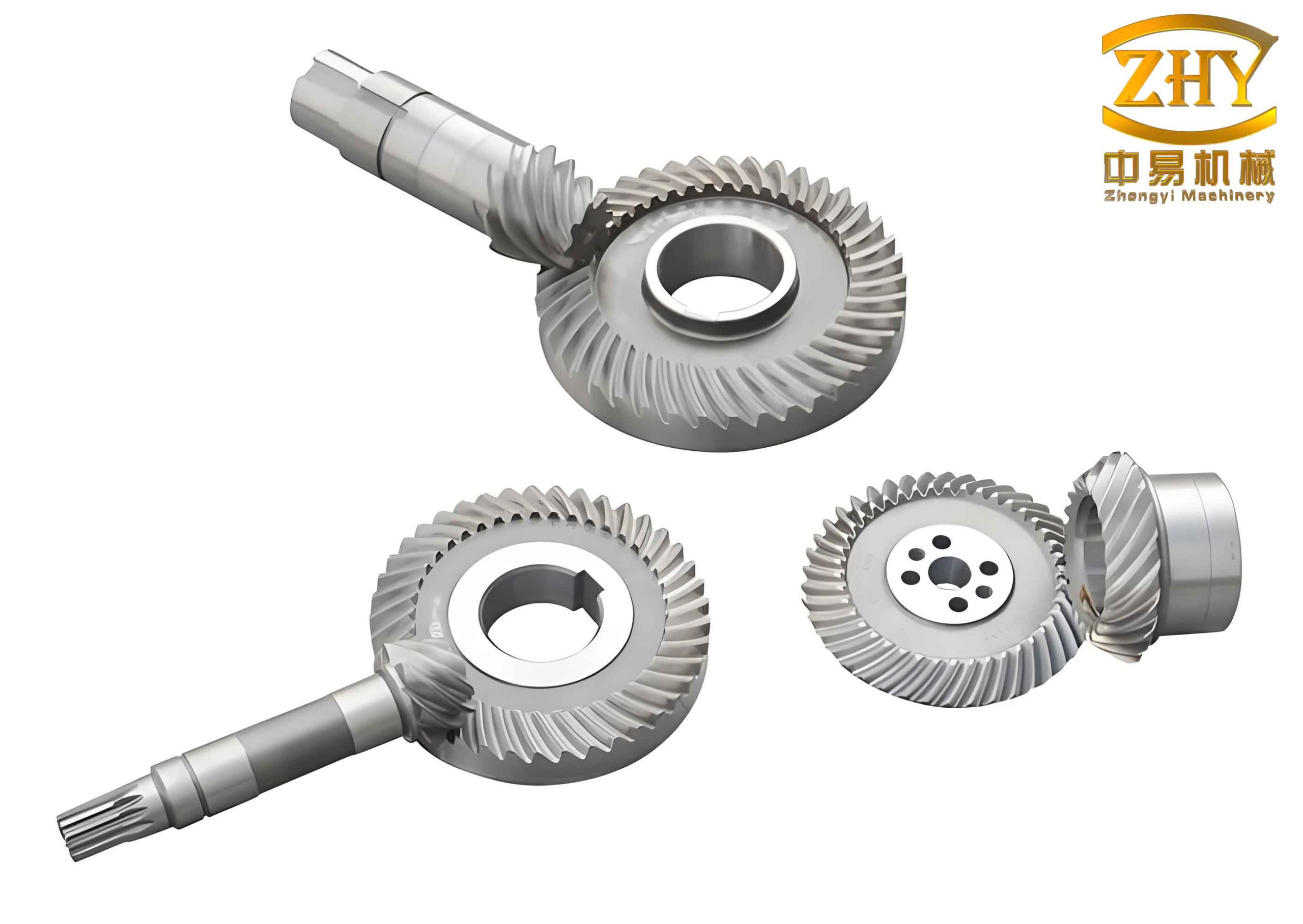
The subsequent phase, parameter design, is where the robust design philosophy is thoroughly applied. Instead of a single-pass optimization, I employ a two-stage process: Direct Optimization (Direct Choice) followed by Stability Optimization. The goal is first to find a promising parameter combination and then to make its performance (the volume \( V \)) insensitive to variations.
For the Direct Optimization, I identified the factors with the most significant influence on the target function: \( z_1 \), \( m_1 \), \( F \), \( E \), and \( \beta_1 \). To explore a broad design space, I assigned seven levels to each factor (except \( z_1 \) and \( m_1 \), which had fewer discrete practical values). This creates a multi-level experimental matrix. An Orthogonal Array \( L_{18}(7^8) \) is an efficient tool to sample this large space with a manageable number of experiments. The factors are assigned to the columns of the array, and for each experimental run (row), the corresponding parameter levels are used to calculate the target volume \( V \). After three iterative rounds of this direct择优 (direct selection) process, analyzing results and refining the level ranges, a promising parameter combination with a relatively small volume was identified. This “good condition” serves as the baseline for the next stage. The result from the third round was: \( z_1=9 \), \( z_2=41 \), \( d_2=190 \, \text{mm} \), \( m_1=6 \), \( F=29 \, \text{mm} \), \( E=32 \, \text{mm} \), \( \beta_1=0.87 \, \text{rad} \), yielding \( V = 857369.5 \, \text{mm}^3 \).
| Level | X1 (z1) | X2 (z2) | X3 (d2/mm) | X4 (m1/mm) | X5 (F/mm) | X6 (E/mm) | X7 (β1/rad) |
|---|---|---|---|---|---|---|---|
| 1 | 7 | 35 | 170 | 5 | 24 | 17 | 0.80 |
| 2 | 8 | 37 | 180 | 6 | 26 | 20 | 0.81 |
| 3 | 8 | 39 | 190 | 7 | 28 | 23 | 0.82 |
| 4 | 9 | 41 | 200 | 7 | 30 | 26 | 0.84 |
| 5 | 9 | 41 | 210 | 7 | 29 | 29 | 0.86 |
| 6 | 10 | 43 | 220 | 8 | 34 | 32 | 0.88 |
| 7 | 10 | 45 | 230 | 9 | 36 | 35 | 0.90 |
The Stability Optimization focuses on making the output robust. From the seven original factors, I now treat \( X_3 (d_2) \), \( X_5 (F) \), and \( X_6 (E) \) as the primary “control factors” to adjust for stability, as the others are often determined by ratio or standardized modules. Each is given three levels centered around the promising values from the direct optimization. This forms the “inner array” using an \( L_9(3^4) \) orthogonal table.
| Level | X3 (d2/mm) | X5 (F/mm) | X6 (E/mm) |
|---|---|---|---|
| 1 | 190 | 6 | 24 |
| 2 | 195 | 7 | 28 |
| 3 | 200 | 8 | 32 |
The critical step here is introducing “noise factors” – the uncontrollable variations in these very same parameters and others during manufacturing and assembly. For each of the 9 experimental conditions in the inner array, I create a corresponding “noise factor table” (outer array). For example, the noise factors \( X’_3 \), \( X’_5 \), and \( X’_6 \) (representing the actual manufactured values) are assigned levels like ±1%, ±5%, and ±6% around their nominal values specified in the inner array. An \( L_9(3^4) \) array is also used for this outer design. For each inner-outer combination, the volume \( V \) is recalculated.
This generates nine output values \( Y_i \) (i=1 to 9) for each of the nine inner array conditions. Rather than just averaging these, I use the Signal-to-Noise (SN) Ratio, a metric from Taguchi Methods, to evaluate robustness. For a “smaller-the-better” characteristic like volume, the SN ratio \( \eta \) is calculated as:
$$ \eta = -10 \log_{10} \left( \frac{1}{n} \sum_{i=1}^{n} Y_i^2 \right) $$
A higher SN ratio indicates that the mean performance is achieved with minimal variation due to noise factors – the very definition of robustness. I calculate the SN ratio for each of the nine conditions in the inner array. Statistical analysis (ANOVA) of these SN ratios reveals which control factors significantly affect robustness. In this case, factor \( X_6 \) (offset \( E \)) was found to be highly significant, and \( X_5 \) (face width \( F \)) was significant. The optimal levels are chosen to maximize the SN ratio: Level 1 for both \( X_3 \) (190 mm) and \( X_5 \) (6 mm). \( X_6 \) is chosen to also minimize the nominal volume, leading to Level 3 (32 mm). This yields the Optimal Robust Parameter Set.
| Factor | Parameter | Optimal Nominal Value |
|---|---|---|
| X1 | Pinion Teeth (z1) | 9 |
| X2 | Gear Teeth (z2) | 41 |
| X3 | Gear Pitch Diameter (d2) | 190 mm |
| X4 | Face Module (m1) | 6 mm |
| X5 | Face Width (F) | 29 mm |
| X6 | Offset (E) | 32 mm |
| X7 | Spiral Angle (β1) | 0.87 rad (~49.8°) |
Nominal Target Volume, V: 857369.5 mm³
The final stage is Tolerance Design. Now that the best nominal values are known, the question becomes: what manufacturing tolerances are economically justified? I start by establishing an error factor table around the optimal nominal values, typically using ±3σ limits corresponding to a standard machining precision grade.
| Level | X’3 (d2/mm) | X’5 (F/mm) | X’6 (E/mm) | X’7 (β1/rad) |
|---|---|---|---|---|
| 1 | 189.05 | 28.55 | 31.04 | 0.868 |
| 2 (Nominal) | 190.00 | 29.00 | 32.00 | 0.870 |
| 3 | 190.95 | 29.45 | 32.96 | 0.872 |
Another outer array experiment (using \( L_9 \)) is performed with these error factors. The resulting variance in the output volume \( V \) is analyzed to determine the contribution of each error factor to the total variation. The analysis showed that \( X’_3 \) (diameter variation) contributed 54.8%, \( X’_6 \) (offset variation) 3.8%, and \( X’_5 \) (face width variation) 9.3% to the output variance.
To decide if tolerances should be tightened, I consider the economic trade-off using a quadratic loss function. The loss \( L(y) \) due to deviation from the nominal target \( m \) is modeled as:
$$ L(y) = k (y – m)^2 $$
where \( k \) is a proportionality constant, \( y \) is the actual volume, and \( m = 857369.5 \, \text{mm}^3 \). The expected loss under the current variation is proportional to the variance \( \sigma^2 \). The question is whether reducing the variance (by tightening the tolerance on the major contributor, \( X’_3 \)) justifies the increased manufacturing cost. In this specific case, the analysis concluded that halving the tolerance on \( d_2 \) would not provide sufficient reduction in expected quality loss to offset the significant increase in machining cost and difficulty. Therefore, the standard commercial tolerances are deemed acceptable. This completes the robust design cycle.
| Design Parameter | Symbol | Nominal Value | Tolerance |
|---|---|---|---|
| Pinion Teeth | \( z_1 \) | 9 | – |
| Gear Teeth | \( z_2 \) | 41 | – |
| Gear Pitch Diameter | \( d_2 \) | 190.0 mm | ±0.95 mm |
| Face Module | \( m_1 \) | 6.0 mm | – |
| Face Width | \( F \) | 29.0 mm | ±0.45 mm |
| Offset | \( E \) | 32.0 mm | ±0.96 mm |
| Spiral Angle | \( \beta_1 \) | 0.870 rad | ±0.002 rad |
In conclusion, the robust optimization design method provides a powerful and systematic framework for designing automotive final drive hypoid gears. It moves beyond finding a merely optimal nominal point to finding a parameter set that maintains consistent, high-quality performance in the face of real-world manufacturing variations. This methodology successfully addresses the limitations of both traditional experiential design and conventional deterministic optimization. The resulting design is not only volume-efficient but also manufacturable and reliable. The parameters determined through this process do not require subsequent rounding or standardization, making the results directly applicable for engineering and production. This approach holds significant practical value for improving the quality and accelerating the localization of automotive powertrain components, ensuring that robust and efficient hypoid gear designs are consistently achieved.