
In modern industrial automation, the widespread adoption of industrial robots has underscored the critical need for reliable and efficient fault diagnosis systems. Among key components, the RV reducer plays a pivotal role due to its high precision, compact structure, large reduction ratio, and robust load-bearing capacity. However, operating under harsh conditions such as heavy loads and frequent speed variations can degrade the performance of the RV reducer, leading to system failures, unplanned downtime, and economic losses. Traditional fault diagnosis methods for gear reducers often rely on vibration signals, which, while effective, face practical limitations including sensor installation constraints, signal interference, and challenges in variable-speed conditions. To address these issues, motor current signal analysis (MCSA) has emerged as a promising alternative, offering non-invasive, cost-effective monitoring. Nevertheless, extracting meaningful fault features from current signals remains challenging due to weak fault signatures and complex noise environments. In this study, we propose a novel fault feature extraction method combining MCSA, sparse autoencoder (SAE), and Fisher criterion for RV reducer fault diagnosis. This approach leverages deep learning to autonomously learn discriminative features from current signal spectra, enhancing diagnostic accuracy and robustness. We validate the method through experiments on an RV reducer test bench, demonstrating superior performance compared to classical machine learning techniques.
The core of our method lies in the integration of SAE for unsupervised feature learning and Fisher criterion for feature selection. SAE, a variant of autoencoder, introduces sparsity constraints to learn compact and informative representations from input data. Given an input vector \( \mathbf{x} \in \mathbb{R}^l \), the encoding process produces a hidden representation \( \mathbf{h} \) through a nonlinear transformation: $$ \mathbf{h} = f(\mathbf{W} \mathbf{x} + \mathbf{b}), $$ where \( f \) is an activation function (e.g., sigmoid), \( \mathbf{W} \) is a weight matrix, and \( \mathbf{b} \) is a bias vector. The decoder reconstructs the input as \( \mathbf{y} = f(\mathbf{h} \mathbf{W}^T + \mathbf{c}) \). To promote sparsity, a penalty term based on Kullback-Leibler divergence is added to the cost function: $$ J_{\text{sparse}}(\mathbf{W}, \mathbf{b}) = \frac{1}{N} \sum_{i=1}^{N} \frac{1}{2} \| \mathbf{h}_{\mathbf{W},\mathbf{b}}(\mathbf{x}^{(i)}) – \mathbf{y}^{(i)} \|^2 + \beta \sum_{j=1}^{s_2} \text{KL}(\rho \| \rho_j) + \frac{\gamma}{2} \sum_{l=1}^{2} \sum_{i=1}^{s_l} \sum_{j=1}^{s_{l+1}} (W_{ji}^{(l)})^2, $$ where \( \beta \) controls the sparsity penalty weight, \( \gamma \) is a weight decay coefficient, \( \rho \) is the sparsity parameter, and \( \rho_j \) is the average activation of hidden neuron \( j \). This formulation enables the SAE to extract salient features from frequency-domain signals of RV reducer current data.
To refine the feature set, we apply the Fisher criterion, which evaluates the discriminative power of each feature by computing the ratio of between-class scatter to within-class scatter. For feature \( f \) across \( M \) classes, the Fisher score is defined as: $$ \text{Fscore}(f) = \frac{S_B^f}{S_W^f}, $$ where \( S_B^f = \sum_{i=1}^{M} m_i (\mu_i – \mu)^2 \) is the between-class scatter, \( S_W^f = \frac{1}{N} \sum_{i=1}^{M} \sum_{j \in T_i} (f_{ij} – \mu_i)^2 \) is the within-class scatter, \( \mu_i \) is the mean of feature \( f \) in class \( i \), \( \mu \) is the overall mean, and \( m_i \) is the number of samples in class \( i \). Features with higher Fisher scores are more effective for classification. By ranking features based on their scores and selecting the top \( n \), we obtain an optimal feature subset that enhances diagnostic efficiency. This combination, referred to as Fisher-SAE, allows for automatic feature extraction and selection from RV reducer current signals, overcoming the limitations of manual feature engineering.
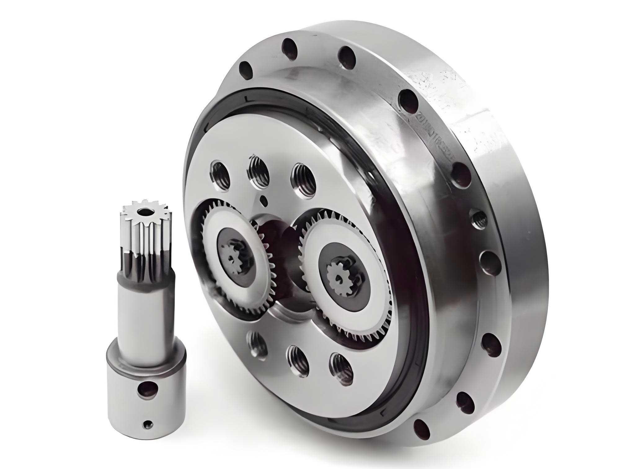
Our experimental setup involved a dedicated RV reducer fault test bench designed to simulate real-world operating conditions. The bench comprised a servo motor, an RV reducer (model 150BX-141-RVE-19), a servo drive, a controller, and a load swing arm. The RV reducer, a critical component in many robotic joints, was driven by the motor to perform 90-degree reciprocating motions at a speed of 100°/s, mimicking typical robot arm movements. Two load conditions were tested: no load (Load 1) and an 8 kg load (Load 2). We examined seven health states of the RV reducer: six fault types and one normal state. The fault types included sun gear root crack, sun gear single-tooth wear, sun gear multi-tooth wear, planetary gear root crack, planetary gear single-tooth wear, and planetary gear multi-tooth wear. These faults were manufactured to replicate realistic damage scenarios in RV reducers. Current signals from the drive motor were sampled at a high frequency, and data segments of 2048 points were extracted for analysis. Each state yielded 300 samples, resulting in a dataset of 7 × 300 × 2048. After normalizing the signals, we computed their frequency spectra via Fast Fourier Transform (FFT) to capture spectral characteristics relevant to RV reducer faults.
The Fisher-SAE method was implemented with a network architecture of [2048, 512, 256, 7], corresponding to the input layer, two hidden layers, and a SoftMax output layer. We investigated the impact of hyperparameters, specifically the sparsity penalty weight \( \beta \) and sparsity parameter \( \rho \), on diagnostic accuracy. Through grid search, optimal values were determined as \( \beta = 7 \) and \( \rho = 0.35 \), maximizing the classification performance. The SAE was trained in two stages: unsupervised pre-training to initialize weights, followed by supervised fine-tuning using backpropagation. Features extracted from the hidden layers were then evaluated using the Fisher criterion. The ranking of Fisher scores revealed significant variation in discriminative power among features, as summarized in Table 1. For instance, the top-ranked feature had a score approximately 16 times higher than the lowest-ranked one, justifying the need for feature selection. By selecting the top 60 features based on Fisher scores, we formed an optimal feature set that improved both accuracy and computational efficiency.
| Feature Rank | Fisher Score Range | Discriminative Category |
|---|---|---|
| Top 30 Features | 15.2 – 24.8 | High |
| Bottom 30 Features | 0.5 – 1.8 | Low |
The diagnostic results under both load conditions demonstrated the efficacy of the Fisher-SAE method. For Load 1, the classification accuracy achieved 100% with zero standard deviation across multiple trials, indicating perfect separation of all seven RV reducer states. The confusion matrix confirmed that every test sample was correctly classified. Similarly, under Load 2, the method maintained 100% accuracy, showcasing its robustness to varying operational loads. Visualizations using t-distributed stochastic neighbor embedding (t-SNE) illustrated clear clustering of samples by fault type for the top 60 features, whereas the bottom 60 features resulted in overlapping clusters, as shown in Table 2. This contrast underscores the importance of feature selection in enhancing the diagnostic capability for RV reducer faults.
| Feature Set | Clustering Separation | Diagnostic Accuracy |
|---|---|---|
| Top 60 Features (Fisher-selected) | Well-separated clusters | 100% |
| Bottom 60 Features | Overlapping clusters | < 50% (estimated) |
To further validate our approach, we compared Fisher-SAE with classical machine learning methods commonly used in fault diagnosis, including support vector machine (SVM), k-nearest neighbors (KNN), discriminant analysis (DA), naive Bayes (NB), and decision trees (DT). These methods relied on manually extracted frequency-domain features, such as mean, variance, skewness, kurtosis, and spectral peaks, totaling 16 traditional features. The comparison was conducted under both load conditions, with results averaged over 15 runs to ensure statistical reliability. As presented in Table 3, Fisher-SAE outperformed all classical methods, achieving perfect accuracy, while the best classical method, SVM, reached only 94.9% under Load 2 and 83.1% under Load 1. This performance gap highlights the limitations of handcrafted features in capturing complex fault patterns in RV reducer current signals, especially under light loads where fault signatures are more subtle.
| Method | Load 1 Accuracy (%) | Load 2 Accuracy (%) | Standard Deviation |
|---|---|---|---|
| Decision Tree (DT) | 77.57 | 84.37 | ±2.5 |
| Discriminant Analysis (DA) | 83.85 | 93.75 | ±1.8 |
| Naive Bayes (NB) | 84.00 | 90.18 | ±2.2 |
| Support Vector Machine (SVM) | 83.10 | 94.90 | ±1.5 |
| K-Nearest Neighbors (KNN) | 81.50 | 94.00 | ±2.0 |
| Fisher-SAE (Proposed) | 100.00 | 100.00 | ±0.0 |
The superior performance of Fisher-SAE can be attributed to its ability to learn hierarchical representations directly from raw frequency-domain data, eliminating the need for domain-specific feature engineering. The SAE component adaptively extracts deep features that encapsulate nonlinear relationships and subtle fault indicators in RV reducer current signals. Subsequently, the Fisher criterion refines these features by selecting the most discriminative subset, reducing redundancy and enhancing generalization. This is particularly beneficial for RV reducers, where faults like gear cracks or wear manifest as faint modulations in motor current spectra. Moreover, the method’s invariance to load variations demonstrates its potential for real-world applications where operating conditions fluctuate. Mathematical analysis of the feature extraction process can be extended by considering the spectral characteristics of RV reducer faults. For example, fault-induced frequency components \( f_{\text{fault}} \) in current signals can be modeled as: $$ f_{\text{fault}} = f_s \pm k \cdot f_r, $$ where \( f_s \) is the supply frequency, \( f_r \) is the rotational frequency of the RV reducer, and \( k \) is an integer. The SAE learns to detect these components without explicit formulation, enabling robust diagnosis.
In terms of computational efficiency, the Fisher-SAE method offers a balance between accuracy and resource usage. The training phase, though iterative, is performed offline, while the online diagnosis involves only forward propagation through the network and feature selection, ensuring rapid response. To quantify this, we estimated the time complexity of key steps: SAE feature extraction scales with \( O(n \cdot m) \) where \( n \) is the number of samples and \( m \) is the feature dimension, while Fisher scoring requires \( O(n \cdot d) \) for \( d \) features. In practice, for our RV reducer dataset, the entire process completed within seconds on standard hardware. This efficiency makes the method suitable for continuous monitoring of industrial robots equipped with RV reducers. Additionally, the modular design allows for integration with other signal types, such as vibration or temperature data, though MCSA remains advantageous due to its non-invasive nature.
Despite its successes, the Fisher-SAE method has limitations that warrant future research. The performance depends on hyperparameter tuning, which may require domain expertise or automated optimization techniques like Bayesian optimization. Furthermore, the current study focused on seeded faults in a controlled environment; real-world RV reducer faults might involve more complex patterns or multiple concurrent faults. Expanding the method to handle such scenarios, perhaps through multi-label classification or anomaly detection, would enhance its applicability. Another direction is to incorporate explainable AI techniques to interpret the learned features, providing insights into the physical mechanisms of RV reducer faults. For instance, visualizing the weight matrices of the SAE could reveal which frequency bands are most sensitive to specific faults, aiding in preventive maintenance.
In conclusion, we have developed and validated a fault feature extraction method based on MCSA and Fisher-SAE for RV reducer diagnosis. This approach effectively overcomes the limitations of vibration-based methods and traditional feature extraction by leveraging deep learning to autonomously derive discriminative features from motor current signals. Experimental results on an RV reducer test bench show that Fisher-SAE achieves 100% diagnostic accuracy across multiple fault types and load conditions, outperforming classical machine learning methods by a significant margin. The integration of SAE for feature learning and Fisher criterion for feature selection ensures both robustness and efficiency, making it a promising tool for real-time health monitoring of RV reducers in industrial robots. Future work will focus on extending the method to more diverse fault scenarios and operational environments, further solidifying its role in advancing the reliability of automation systems.
To summarize the mathematical foundations, key equations governing the Fisher-SAE method include the SAE cost function: $$ J_{\text{sparse}} = \frac{1}{N} \sum_{i=1}^{N} \frac{1}{2} \| \mathbf{h}(\mathbf{x}^{(i)}) – \mathbf{y}^{(i)} \|^2 + \beta \sum_{j=1}^{s_2} \left( \rho \log \frac{\rho}{\rho_j} + (1-\rho) \log \frac{1-\rho}{1-\rho_j} \right) + \frac{\gamma}{2} \sum_{l} \sum_{i,j} (W_{ji}^{(l)})^2, $$ and the Fisher score: $$ \text{Fscore} = \frac{\sum_{i=1}^{M} m_i (\mu_i – \mu)^2}{\frac{1}{N} \sum_{i=1}^{M} \sum_{j \in T_i} (f_{ij} – \mu_i)^2}. $$ These formulations enable effective feature extraction and selection for RV reducer fault diagnosis, contributing to the broader goal of intelligent maintenance in industrial automation.