
The reliability of industrial robots is fundamentally tied to the performance of their core components, with the rotary vector reducer being one of the most critical. Positioned at the robot’s joints, this reducer is responsible for transmitting motion and torque with high precision and under significant load. Its longevity and consistent performance directly dictate the operational lifespan and accuracy of the entire robotic system. However, the rotary vector reducer is characterized by an exceptionally long life and slow degradation under normal operating conditions. Conducting full life-cycle tests to assess its reliability is prohibitively time-consuming and costly. This study addresses this challenge by proposing and executing a high-stress accelerated degradation test (ADT) on rotary vector reducers. We utilize transmission accuracy as the key performance indicator and model its degradation using a Wiener stochastic process, ultimately deriving a reliability function for the rotary vector reducer that accounts for unit-to-unit variability even with a small sample size.
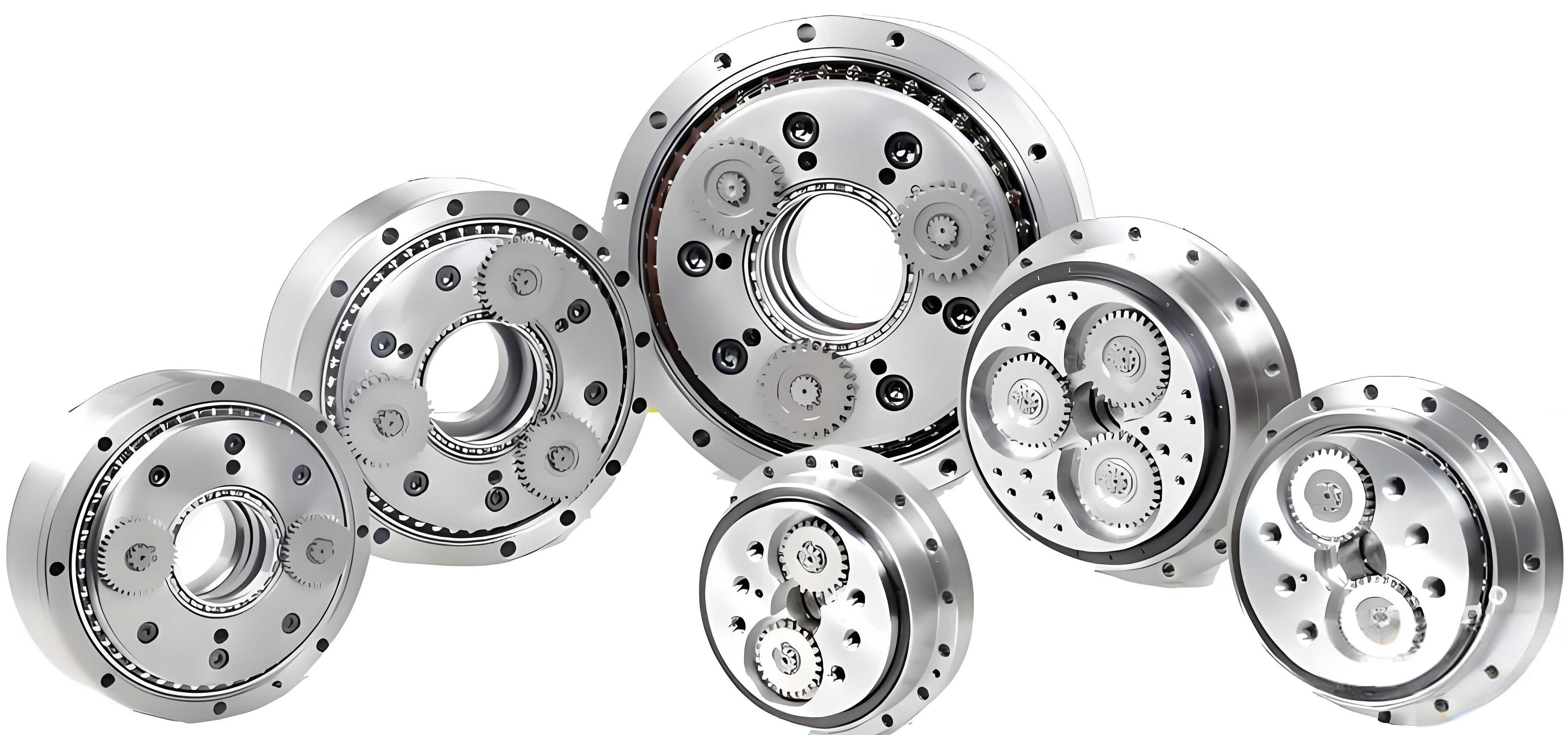
The rotary vector reducer achieves its capabilities through a unique two-stage transmission mechanism housed within a compact structure. The first stage consists of a planetary gear train. An input shaft, connected to a servomotor, drives two or three planetary gears. The second stage is a cycloid-pin gear mechanism. The planetary gears drive crankshafts, which cause eccentric motion in cycloid discs. These discs mesh with a ring of stationary pins housed in a pin gear casing, generating a high reduction ratio. The motion is finally output through an output flange. This combination provides the rotary vector reducer with its renowned advantages: a large reduction ratio, high torsional stiffness, compact size, and excellent positioning accuracy.
Transmission accuracy, defined as the deviation between the theoretical and actual output rotation angle, is the paramount performance metric for a rotary vector reducer. Its degradation over time directly translates to a loss in robot positioning precision. Therefore, this study selects transmission accuracy as the degradation characteristic for reliability assessment. The failure threshold is defined as a degradation of 20 arcseconds from the initial performance value.
High-Stress Accelerated Degradation Testing Platform and Principle
To efficiently gather degradation data, a dedicated test platform was constructed. The platform’s core principle involves driving the rotary vector reducer under controlled, elevated stress conditions while continuously monitoring its performance. An input servomotor provides the driving rotation, while an output servomotor applies a constant, high-magnitude braking torque to simulate an extreme operational load. This configuration applies a steady, high stress, which effectively accelerates the wear and degradation processes within the rotary vector reducer compared to the fluctuating loads typical of swing-arm type testers.
Sensors are integral to the platform. High-resolution rotary encoders are mounted on both the input and output shafts to measure angular position. Torque and speed sensors monitor the operational parameters. A dedicated data acquisition system, controlled via LabVIEW software, collects sensor readings at specified intervals. The transmission accuracy is calculated in real-time from the difference between the expected output angle (based on the input and the nominal reduction ratio) and the measured output angle.
Strength Verification for Determining Maximum Test Load
A critical step before conducting an accelerated test is to determine the maximum applicable stress level that does not alter the fundamental failure mechanisms. For the rotary vector reducer, the cycloid-pin gear transmission is identified as a potential weak link due to its complex contact mechanics and high load concentration. Therefore, a theoretical strength verification of this subsystem was performed at 2.5 times the rated torque to justify the selected accelerated stress level.
The analysis accounts for profile modifications applied to the cycloid tooth flank, which are standard in manufacturing to compensate for errors and ensure lubrication. The initial clearance $\Delta(\varphi_i)$ between a modified cycloid tooth and a pin tooth at angle $\varphi_i$ is given by:
$$
\Delta(\varphi_i) = \Delta r_{rp}\left(1 – \frac{\sin \varphi_i}{\sqrt{1 + K_1^2 – 2K_1\cos \varphi_i}}\right) + \frac{\Delta r_p\left(1 – K_1\cos \varphi_i – \sqrt{1 – K_1^2}\sin \varphi_i\right)}{\sqrt{1 + K_1^2 – 2K_1\cos \varphi_i}}
$$
where $\Delta r_{rp}$ is the offset modification, $\Delta r_p$ is the equidistant modification, and $K_1 = e z_p / r_p$ is the shortening coefficient.
Under an applied output torque $T$, the total deformation $\delta_i$ along the common normal at a potential contact point is proportional to its distance $l_i$ from the center of the cycloid disc:
$$
\delta_i = l_i \beta = \frac{\sin \varphi_i}{\sqrt{1 + K_1^2 – 2K_1\cos \varphi_i}} \delta_{max}
$$
where $\beta$ is the angular deflection of the cycloid disc and $\delta_{max}$ is the maximum deformation, composed of Hertzian contact deformation $\omega_{max}$ and pin bending deformation $f_{max}$.
The contact deformation is calculated using the Hertz formula:
$$
\omega_{max} = \frac{2 F_{max}}{\pi L} \left[ \frac{1-\mu_1^2}{E_1} \left( \frac{1}{3} + \ln\frac{4R_1}{c} \right) + \frac{1-\mu_2^2}{E_2} \left( \frac{1}{3} + \ln\frac{4R_2}{c} \right) \right]
$$
and
$$
c = 1.60 \sqrt{ \frac{F_{max}}{L} K_D \left( \frac{1-\mu_1^2}{E_1} + \frac{1-\mu_2^2}{E_2} \right) }
$$
The pin bending deformation is approximated using beam theory:
$$
f_{max} = \frac{31}{64} \cdot \frac{F_{max} L^3}{48 E J}
$$
A tooth pair enters contact only if the total deformation exceeds the initial clearance: $\delta_i – \Delta(\varphi_i) > 0$. The force on each contacting tooth $i$ is then:
$$
F_i = \frac{\delta_i – \Delta(\varphi_i)}{\omega_{max}} F_{max}
$$
The maximum force $F_{max}$ is found iteratively by solving the equilibrium equation between the sum of moments from all contacting teeth and the transmitted torque $T_C$ per cycloid disc ($T_C \approx 0.55T$):
$$
T_C = \sum_{i \in \text{contact}} F_i \cdot l_i = \sum_{i \in \text{contact}} \left( \frac{l_i}{r’_c} – \frac{\Delta(\varphi_i)}{\omega_{max}} \right) l_i \cdot F_{max}
$$
Finally, the contact stress $\sigma_{H}$ for each meshing tooth is calculated:
$$
\sigma_{H} = 0.418 \sqrt{ \frac{E_d F_i}{b_c \rho_{ei}} }
$$
where $E_d$ is the equivalent elastic modulus and $\rho_{ei}$ is the equivalent curvature radius at the contact point.
Performing this analysis for a specific rotary vector reducer model at 412 Nm (2.5 times its rated 167 Nm torque) yielded the following results for the load distribution and contact stress:
| Pin Tooth Number | Engagement Force $F_i$ (N) | Contact Stress $\sigma_H$ (MPa) |
|---|---|---|
| 2 | 362.7743 | 883.8431 |
| 3 | 549.7524 | 1094.8284 |
| 4 | 598.0550 | 1144.0783 |
| 5 | 600.9939 | 1147.9370 |
| 6 | 583.8370 | 1132.0442 |
| 7 | 555.3172 | 1104.4417 |
| 8 | 519.2143 | 1068.2065 |
| 9 | 477.4945 | 1024.5848 |
| 10 | 431.3543 | 973.9668 |
| 11 | 381.6269 | 916.2144 |
| 12 | 328.9606 | 850.7281 |
| 13 | 273.9033 | 776.3360 |
| 14 | 216.9463 | 690.9684 |
| 15 | 158.5473 | 590.7263 |
| 16 | 99.1430 | 467.1531 |
| 17 | 39.1554 | 293.5910 |
The results show that 16 teeth share the load simultaneously, with the maximum contact stress of approximately 1148 MPa occurring at tooth #5. This stress is below the allowable contact stress for the cycloid disc material (20CrMnMo, ~1268 MPa) and the pin material (GCr15, ~3636 MPa). This verification confirmed that a load of 412 Nm does not cause instantaneous yield or fracture, validating its use as an elevated stress level for accelerated degradation without changing the underlying wear and fatigue failure modes.
Accelerated Degradation Test Execution and Results
Based on the strength verification, a high-stress accelerated degradation test was designed and carried out. The accelerated stress selected was output load torque. Three identical RV-20E rotary vector reducers were tested under identical conditions: an input speed of 1815 rpm and a constant output load torque of 412 Nm. The transmission accuracy was measured at regular intervals. The raw degradation data (increase in transmission error) collected over time is summarized below:
| Time (h) | Unit 1 $y^{(1)}$ (arcsec) | Time (h) | Unit 2 $y^{(2)}$ (arcsec) | Time (h) | Unit 3 $y^{(3)}$ (arcsec) |
|---|---|---|---|---|---|
| 12 | 4.06 | 12 | 3.58 | 8 | 4.16 |
| 24 | 4.13 | 24 | 3.84 | 16 | 4.85 |
| 36 | 5.13 | 36 | 4.04 | 24 | 5.15 |
| 52 | 7.23 | 48 | 4.04 | 32 | 6.19 |
| 68 | 6.73 | 60 | 6.57 | 40 | 6.32 |
| 82 | 4.76 | 72 | 6.93 | 48 | 7.35 |
| 96 | 4.48 | 84 | 5.23 | 56 | 6.95 |
| 110 | 6.30 | 96 | 6.89 | 64 | 6.89 |
| 124 | 6.28 | 108 | 8.58 | 72 | 6.11 |
| 140 | 8.21 | 120 | 8.67 | 80 | 5.62 |
| 156 | 8.98 | 132 | 10.60 | 88 | 6.41 |
| 172 | 7.04 | 144 | 11.36 | 96 | 7.06 |
| 188 | 9.95 | 156 | 13.10 | 104 | 9.00 |
| 204 | 11.76 | 168 | 12.71 | 112 | 9.46 |
| – | – | 180 | 16.16 | 120 | 9.98 |
The data clearly shows an accelerating degradation trend for all three units, confirming the effectiveness of the high-stress test. Notably, a temporary recovery or “resilience” period is observed between 60-100 hours, where the transmission accuracy slightly improves. This is attributed to a running-in process where initial friction and settling of components lead to a more optimal operating state. Crucially, the data exhibits inherent unit-to-unit variability; Unit 2 degrades at a faster rate than Units 1 and 3, highlighting the individual differences arising from manufacturing and assembly tolerances.
To model reliability under normal conditions, the accelerated test time $t$ and load $T_m$ need to be converted to equivalent operating hours $L_h$ at the rated load $T_0$ using a fatigue equivalence formula based on the $10/3$ power law for bearing-like components:
$$
L_h = t \times \frac{N_0}{N_m} \times \left( \frac{T_0}{T_m} \right)^{10/3}
$$
Applying this conversion transforms the accelerated degradation paths into equivalent degradation trends under normal rated load (167 Nm, 15 rpm output), providing the foundational data for reliability modeling under use conditions.
Degradation Modeling Using Wiener Process
The Wiener process is a suitable stochastic model for the degradation of rotary vector reducers because it naturally incorporates both a monotonic degradation trend and random temporal fluctuations, which are evident in the test data. The Wiener process model for performance degradation $y(t)$ is given by:
$$
y(t) = \alpha + \mu t + \sigma B(t)
$$
where:
$\alpha$ is the initial degradation offset at $t=0$,
$\mu$ is the drift coefficient representing the average degradation rate,
$\sigma$ is the diffusion coefficient representing the magnitude of random fluctuations, and
$B(t)$ is a standard Brownian motion with $B(t) \sim N(0, t)$ and independent increments.
For a failure threshold $D_f$, the first-passage time $T$ when $y(t) \geq D_f$ follows an Inverse Gaussian (IG) distribution. The probability density function (PDF) and reliability function $R(t)$ are:
$$
f(t | \alpha, \mu, \sigma) = \frac{D_f – \alpha}{\sqrt{2\pi \sigma^2 t^3}} \exp\left( -\frac{(D_f – \alpha – \mu t)^2}{2\sigma^2 t} \right)
$$
$$
R(t | \alpha, \mu, \sigma) = \Phi\left( \frac{D_f – \alpha – \mu t}{\sigma \sqrt{t}} \right) – \exp\left( \frac{2\mu(D_f – \alpha)}{\sigma^2} \right) \Phi\left( \frac{-(D_f – \alpha) – \mu t}{\sigma \sqrt{t}} \right)
$$
where $\Phi(\cdot)$ is the standard normal cumulative distribution function.
Parameter Estimation for Individual Units
To capture unit-to-unit variability, the parameters $(\alpha_i, \mu_i, \sigma_i)$ are estimated separately for each rotary vector reducer $i$ using the maximum likelihood estimation (MLE) method with separated sample data. For a unit with measurements $y_1, y_2, …, y_N$ at times $t_1, t_2, …, t_N$, the increments $\Delta y_k = y_{k+1} – y_k$ are independent and normally distributed: $\Delta y_k \sim N(\mu \Delta t_k, \sigma^2 \Delta t_k)$ for $k \geq 1$, and $y_1 \sim N(\alpha + \mu t_1, \sigma^2 t_1)$.
The MLE estimates derived from the likelihood function are:
$$
\hat{\mu}_i = \frac{1}{N} \sum_{k=1}^{N} \frac{\Delta y_k}{\Delta t_k}, \quad \hat{\sigma}_i = \sqrt{ \frac{1}{N} \sum_{k=1}^{N} \frac{(\Delta y_k – \hat{\mu}_i \Delta t_k)^2}{\Delta t_k} }, \quad \hat{\alpha}_i = y_1 – \hat{\mu}_i t_1
$$
Applying this to the converted degradation data from the three rotary vector reducers yields the following unit-specific parameters:
| Unit $i$ | Initial Degradation $\hat{\alpha}_i$ (arcsec) | Drift Coefficient $\hat{\mu}_i$ (arcsec/h) | Diffusion Coefficient $\hat{\sigma}_i$ (arcsec/√h) |
|---|---|---|---|
| 1 | 4.0386 | 0.0017 | 0.0110 |
| 2 | 3.5368 | 0.0036 | 0.0110 |
| 3 | 4.1416 | 0.0023 | 0.0123 |
Population Reliability Analysis with Small Sample Size
Directly using the three sets of parameters in the IG distribution would require complex integration over the joint distribution of $(\alpha, \mu, \sigma)$. To simplify and create a population reliability model from this small sample, we analyze the variability of each parameter. The coefficient of variation (CV) indicates which parameter exhibits the most significant unit-to-unit variation:
$$
CV(X) = \frac{\sqrt{Var(X)}}{E(X)}
$$
Calculating the sample mean, variance, and CV for each parameter:
| Statistic | $\alpha$ | $\mu$ | $\sigma$ |
|---|---|---|---|
| Mean $E(X)$ | 3.9057 | 0.0025 | 0.0114 |
| Variance $Var(X)$ | 0.0698 | 6.300e-7 | 3.767e-6 |
| Coefficient of Variation $CV(X)$ | 0.0698 | 0.3175 | 0.0538 |
The drift coefficient $\mu$ has the largest coefficient of variation (0.3175), indicating the most significant variation in degradation rates among units. The initial degradation $\alpha$ and diffusion coefficient $\sigma$ are relatively stable. Therefore, for the population model, we treat $\alpha$ and $\sigma$ as fixed at their sample means ($\bar{\alpha}=3.9057$, $\bar{\sigma}=0.0114$), and model $\mu$ as a normally distributed random variable representing unit heterogeneity: $\mu \sim N(\bar{\mu}=0.0025, \delta_{\mu}^2 = (7.9373 \times 10^{-4})^2)$.
The unconditional reliability function for the rotary vector reducer population is then obtained by integrating the conditional reliability function $R(t|\mu)$ over the distribution of $\mu$:
$$
R(t) = k \int_{\bar{\mu}-3\delta_{\mu}}^{\bar{\mu}+3\delta_{\mu}} \left[ \Phi\left( \frac{D_f – \bar{\alpha} – \mu t}{\bar{\sigma} \sqrt{t}} \right) – \exp\left( \frac{2\mu(D_f – \bar{\alpha})}{\bar{\sigma}^2} \right) \Phi\left( \frac{-(D_f – \bar{\alpha}) – \mu t}{\bar{\sigma} \sqrt{t}} \right) \right] p(\mu) d\mu
$$
where $p(\mu)$ is the PDF of $N(\bar{\mu}, \delta_{\mu}^2)$, and $k = 1 / [2\Phi(3)-1]$ is a compensation factor for integrating over $\pm3\delta_{\mu}$.
Setting the failure threshold $D_f = 20$ arcseconds and evaluating the integral numerically yields the reliability function $R(t)$ and the failure probability density function $f(t)$ for the rotary vector reducer under normal operating conditions. The mean time to failure (MTTF) can be estimated by:
$$
MTTF = E[T] = \int_0^{\infty} R(t) dt
$$
The resulting reliability curve shows that the rotary vector reducer maintains high reliability ($R(t) > 0.9$) for approximately the first 5,000 equivalent operating hours. Beyond this point, reliability declines more rapidly, with a significant increase in failure probability density between 5,000 and 7,000 hours. This behavior aligns with the typical degradation pattern of mechanical systems: an initial stable period followed by an accelerated wear-out phase, potentially driven by the cumulative fatigue damage in components like the cycloid discs and bearings.
Conclusion
This study successfully demonstrates a practical framework for assessing the reliability of high-life, high-reliability components like the rotary vector reducer. By combining rigorous theoretical strength verification to define a safe accelerated stress level, executing a high-stress accelerated degradation test, and employing a Wiener process-based degradation model, we can extract meaningful reliability information from a very small sample size (three units). The method explicitly accounts for individual unit variability by treating the key degradation rate parameter as a random effect. The results provide a quantified reliability function that predicts the lifespan of rotary vector reducers under normal use, identifying a high-reliability period followed by a wear-out phase. This approach offers a viable and efficient alternative to impossibly long full-life tests, providing crucial data for design validation, maintenance planning, and improvement of industrial robotic systems.