
① Simulation conditions
Based on the established 8-DOF coupling dynamic model of helical gear system, Runge Kutta method is used to solve the dynamic response of helical gear system with and without friction, the dynamic response of helical gear system before and after modification, and the influence of different friction coefficients on the dynamic response of helical gear system after modification. The total coincidence degree of helical gear system is 2.73, the friction coefficient is 0.1, the input torque of driving wheel is 300N / m, and the speed of driving wheel is 600r / min. Specific gear parameters.
By comparing the modification results of different modification methods of helical gear, it can be seen that the fluctuation range of static transmission error of helical gear system is the smallest after linear modification of tooth profile. Therefore, this paper selects the linear gear modification results of helical gear profile to analyze the effects of modification and different friction coefficients on the dynamic response of helical gear system. The static transmission error before and after linear profile modification is shown in the figure.
② Solution method
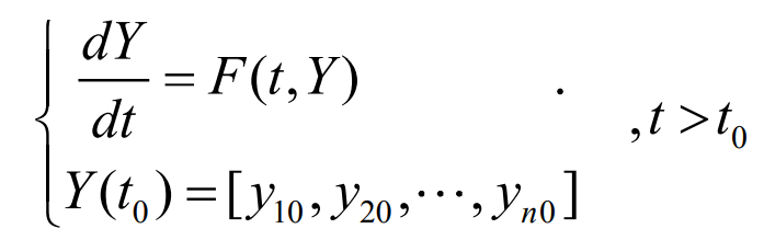
The established helical gear dynamic models include time-varying transmission error and time-varying friction excitation, which belongs to a typical class of strong nonlinear systems. For several approximate methods for solving nonlinear dynamic systems, such as perturbation method, average method and multi-scale method, it is difficult to solve this kind of systems. Only a few very ideal cases can obtain accurate solutions, while most other nonlinear systems can only obtain approximate and numerical solutions. The numerical method overcomes the shortcomings of the above methods. In this paper, the accuracy and efficiency of numerical solution of dynamic differential equation are comprehensively considered. For the dynamic differential equation of helical gear system, the fourth-order Runge Kutta numerical solution is used to solve the micro numerical solution. Runge Kutta method has the advantages of high calculation accuracy, easy programming and good stability. At present, it is a commonly used numerical solution for solving differential equations (Systems) with initial values. The initial value problem of any high-order ordinary differential equation can be transformed into the form of first-order differential equation:
When calculating the function value y, first calculate the point y (T0) respectively. When the value of YN and H are the calculation steps, substitute the calculation results into the calculation formula of the fourth-order Runge Kutta method, and you can get:
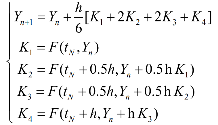
Therefore, the function value yn + 1 is determined by the product of the current value yn plus the step h and the estimated slope. The estimated slope is the weighted average of K1, K2, K3 and K4, where K1 is the time start slope and K2 is the midpoint slope of the time period. The slope K1 is used by Euler method to determine the value of Y at point TN + 0.5h; K3 is also the midpoint slope, and the slope K2 is used to determine the value of Y; K4 is the slope of the end point of the time period, and its y is determined by K3.