
Spur gear transmission systems are widely used in industrial machinery, vehicle transmissions, aerospace actuators, and marine power units because of their simple geometry, high efficiency, and precise transmission ratio. In my research, I focus on tooth surface wear, which is one of the most common gradual fault modes of a spur gear pair. Tooth wear changes the tooth profile, reduces the time-varying mesh stiffness, increases vibration and noise, and eventually leads to gear failure. Therefore, an accurate wear model and a quantitative evaluation method are of great importance for condition monitoring and maintenance of spur gear systems.
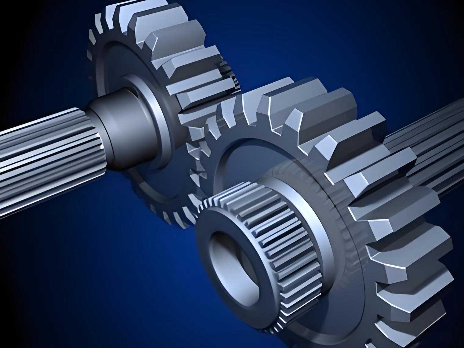
In this thesis, I establish a numerical wear model for a spur gear pair under line-contact mixed elastohydrodynamic lubrication. I also investigate the influence of tooth wear on mesh stiffness and dynamic response. Finally, I propose a quantitative evaluation method for spur gear tooth wear using vibration signal characteristic parameters. The main objectives are to reveal the wear distribution law, investigate the coupling between dynamic load and wear, and provide a practical tool for wear assessment based on vibration measurements.
1. Gear Contact Parameter Calculation for Spur Gear Pairs
I use a standard involute spur gear pair with a contact ratio between 1 and 2 as the research object. The basic geometry of the gear pair is defined by the module \(m\), the tooth numbers \(z_1\) and \(z_2\), the pressure angle \(\alpha\), the addendum coefficient \(h_a\), and the tip clearance coefficient \(C\). The pitch radii of the driving and driven gears are:
$$
r_1 = \frac{m z_1}{2}, \qquad r_2 = \frac{m z_2}{2}
$$
The base circle radii are:
$$
r_{b1} = r_1 \cos\alpha, \qquad r_{b2} = r_2 \cos\alpha
$$
The center distance is \(A = m(z_1 + z_2)/2\). The base pitch is:
$$
p_b = \pi m \cos\alpha
$$
For the gear pair used in my numerical study, the parameters are summarized in Table 1.
| Parameter | Symbol | Value |
|---|---|---|
| Number of teeth of driving gear | \(z_1\) | 18 |
| Number of teeth of driven gear | \(z_2\) | 27 |
| Module | \(m\) | 2 mm |
| Pressure angle | \(\alpha\) | 20° |
| Face width | \(B\) | 30 mm |
| Addendum coefficient | \(h_a\) | 1 |
| Tip clearance coefficient | \(C\) | 0.25 |
| Elastic modulus | \(E\) | 207 GPa |
| Poisson ratio | \(\delta\) | 0.29 |
| Surface hardness | \(H\) | 2.3 GPa |
| Surface roughness | \(\sigma\) | 0.5 μm |
The active line of action is divided into two double-tooth meshing zones and one single-tooth meshing zone. The contact point moves from the tooth root of the driving gear to the tooth tip. At each meshing position, the radius of curvature of the driving gear \(R_1\), the driven gear \(R_2\), and the equivalent radius \(R_z\) are calculated as:
$$
R_1 = r_{b1}\tan\alpha_{k1}, \qquad R_2 = r_{b2}\tan\alpha_{k2}, \qquad \frac{1}{R_z} = \frac{1}{R_1} + \frac{1}{R_2}
$$
1.1 Contact Force and Load Sharing
When the driven gear transmits a torque \(T_{N2}\), the normal force on the tooth flank is:
$$
F_n = \frac{T_{N2}}{r_{b2}}
$$
The load per unit face width is \(W = F_n / B\). In the single-tooth zone, the total load is carried by one tooth pair. In the double-tooth zone, the load is shared by two tooth pairs. I consider the influence of wear-induced backlash change and the time-varying mesh stiffness of both tooth pairs. The unit load in the double-tooth zone is:
$$
W = \frac{F_n}{B}\frac{M_1 + M_2 + \Delta M_2}{M_1 + M_2}
$$
where \(M_1\) and \(M_2\) are the mesh stiffness values of the two tooth pairs, and \(\Delta\) is the equivalent clearance produced by wear. This load-sharing model enables the wear depth to be updated locally along the tooth profile.
Based on Hertzian contact theory, the half-Hertzian contact width and the maximum contact pressure are:
$$
b = \sqrt{\frac{8 W R_z}{\pi E_z}}, \qquad p_{\max} = \frac{2W}{\pi b}
$$
where \(E_z\) is the equivalent elastic modulus. The average contact pressure is:
$$
p_{\rm avg} = \frac{\pi}{4} p_{\max}
$$
1.2 Sliding Velocity and Sliding Distance
Let \(\omega_1\) and \(\omega_2\) be the angular velocities of the driving and driven gears. The tangential velocities are:
$$
v_1 = \omega_1 R_1, \qquad v_2 = \omega_2 R_2
$$
The sliding velocity and the entrainment velocity are:
$$
v_s = |v_1 – v_2|, \qquad v = \frac{v_1 + v_2}{2}
$$
During one mesh cycle, the sliding distance of the driving gear and the driven gear can be approximated by:
$$
L_1 = 2b\left|1 – \frac{v_2}{v_1}\right|, \qquad L_2 = 2b\left|1 – \frac{v_1}{v_2}\right|
$$
The sliding distance is largest near the tooth root and tooth tip, and nearly zero at the pitch point. Because the Hertzian contact half-width changes abruptly at the transition between single-tooth and double-tooth meshing zones, the sliding distance also has an abrupt change at those positions.
2. Mixed Elastohydrodynamic Lubrication Wear Model
In the mixed lubrication regime, the load is carried partly by the lubricant film and partly by contacting asperities. I define the total contact pressure as:
$$
p = p_h + p_a
$$
where \(p_h\) is the hydrodynamic pressure and \(p_a\) is the asperity contact pressure. The average Reynolds equation used in the line-contact mixed EHL model is:
$$
\frac{\partial}{\partial x}\left(\phi_x\frac{\rho h^3}{\eta}\frac{\partial p}{\partial x}\right) = 12v\frac{\partial(\rho h_T)}{\partial x}
$$
where \(\phi_x\) is the pressure flow factor, \(h\) is the film thickness, \(h_T\) is the average gap between the two rough surfaces, and \(\eta\) and \(\rho\) are the lubricant viscosity and density. The pressure flow factor is:
$$
\phi_x = 1 – 0.9\exp\left(-0.56\frac{h}{\sigma}\right)
$$
The film thickness equation includes the rigid body separation \(h_0\), the geometric separation due to curvature, and the elastic deformation \(\delta(x)\):
$$
h(x) = h_0 + \frac{x^2}{2R_z} + \delta(x)
$$
The elastic deformation is calculated by the Boussinesq integral:
$$
\delta(x) = -\frac{2}{\pi E_z}\int_{x_i}^{x_o} p(s)\ln(s-x)^2\,ds
$$
The viscosity and density of the lubricant depend on pressure and temperature. I use a Roelands-type viscosity equation:
$$
\eta = \eta_0\exp\left\{(\ln\eta_0 + 9.67)\left[\left(1+5.1\times10^{-9}p\right)^{0.68}\left(\frac{T-138}{T_0-138}\right)^{-1.1}-1\right]\right\}
$$
and the density-pressure-temperature relation:
$$
\rho = \rho_0\left[1+\frac{0.6p}{1+1.7p}+0.00065(T-T_0)\right]
$$
The load balance equation is:
$$
\int_{x_i}^{x_o} p(x)\,dx = W
$$
To solve the mixed EHL problem efficiently, I adopt the regression formulas proposed by Masjedi and Khonsari. The minimum film thickness is:
$$
\frac{h_{\min}}{R_z} = 1.652 W^{-0.077}U^{0.716}G^{0.695}\left(1+0.026V^{0.185}W^{0.312}U^{-0.809}G^{-0.977}\right)^{-1}
$$
The asperity load ratio is:
$$
L_a = 0.005\ln\left(1+4470V^{0.408}W^{-0.088}U^{-0.103}G^{-0.485}\right)
$$
where \(U\), \(W\), \(G\), and \(V\) are the dimensionless speed, load, material, and hardness parameters. The film thickness ratio is defined as \(\Lambda = h_{\min}/\sigma\), which is used to evaluate the lubrication condition. In my simulations, the film thickness ratio is mostly between 1 and 2.5, indicating that the spur gear pair operates in the mixed lubrication regime.
2.1 Tooth Surface Temperature
Tooth surface temperature affects the lubricant viscosity and density. I calculate the local flash temperature using Tian’s flash temperature theory:
$$
\Delta T = \frac{2bq}{\pi\left(\frac{K_1 v_1^{1/2}}{k_1^{1/2}}+\frac{K_2 v_2^{1/2}}{k_2^{1/2}}\right)}
$$
where \(q\) is the heat generated at the contact point, \(K_i\) are the thermal conductivities, and \(k_i\) are the thermal diffusivities. The heat flux is composed of asperity friction heat and oil film shear heat:
$$
q = f_c v_s p_a + \Lambda_{\lim} v_s p_h
$$
The instantaneous tooth surface temperature is \(T = T_0 + \Delta T\). I use \(T_0 = 315\,K\) in the calculation.
2.2 Archard Wear Equation under Mixed Lubrication
The classical Archard wear model is:
$$
V = \frac{K F L}{H}
$$
where \(V\) is the wear volume, \(K\) is the dimensionless wear coefficient, \(F\) is the normal load, \(L\) is the sliding distance, and \(H\) is the material hardness. Dividing by the contact area gives the wear depth:
$$
h = \frac{K L p}{H}
$$
In mixed lubrication, only the asperity contact contributes significantly to wear. Therefore, I replace the total pressure with the asperity contact pressure:
$$
h = k L p \frac{L_a}{100}\psi
$$
where \(k\) is the dimensional wear coefficient, \(L_a\) is the asperity load ratio expressed as a percentage, and \(\psi\) is the oil-film deficit coefficient:
$$
\psi = 1-\exp\left[-\frac{X}{v_s t_0}\exp\left(-\frac{E_a}{R_g T}\right)\right]
$$
In this equation, \(X\) is the molecular diameter of the lubricant, \(t_0\) is the vibration time of molecules, and \(E_a\) is the adsorption heat. The values used in my simulation are listed in Table 2.
| Parameter | Value |
|---|---|
| Molecular diameter \(X\) | \(3\times10^{-10}\) m |
| Molecular vibration time \(t_0\) | \(3\times10^{-12}\) s |
| Adsorption heat \(E_a\) | \(4.9\times10^4\) J/mol |
I discretize the tooth profile into a finite number of points and update the wear depth after each load cycle. To maintain computational efficiency, I update the tooth profile when the accumulated wear reaches 1 μm. The flow of the wear calculation is shown by the following procedure.
| Parameter | Value |
|---|---|
| Input speed \(n_1\) | 2000 r/min |
| Output torque \(T_{N2}\) | 300 N·m |
| Lubricant viscosity \(\eta_0\) | 0.35 Pa·s |
| Pressure-viscosity coefficient \(\alpha\) | \(2.5\times10^{-8}\) m²/N |
| Limiting shear stress coefficient \(\Lambda_{\lim}\) | 0.0910 |
3. Numerical Results of Spur Gear Tooth Wear
I first analyze the tooth surface contact pressure, sliding distance, lubricant film thickness, asperity contact ratio, and flash temperature along the tooth profile. Then I compute the wear depth for the driving and driven gears.
The main observations from the numerical simulation are as follows:
- The wear depth of the pinion is larger than that of the gear because the pinion rotates more times for the same number of load cycles.
- From tooth root to tooth tip, the wear depth first decreases and then increases. The maximum wear depth of the driving spur gear occurs at the tooth root, while the maximum wear depth of the driven spur gear occurs at the tooth tip.
- The minimum wear depth occurs near the pitch point, where the sliding velocity is almost zero.
- Abrupt changes in wear depth appear at the transitions between single-tooth and double-tooth meshing zones because of the sudden change in load and sliding distance.
Table 4 gives a representative wear distribution for the baseline spur gear pair after \(1\times10^6\) wear cycles.
| Location | Driving gear wear (mm) | Driven gear wear (mm) |
|---|---|---|
| First double-tooth zone near root | \(2.15\times10^{-4}\) | \(1.10\times10^{-4}\) |
| Single-tooth zone start | \(1.05\times10^{-4}\) | \(0.72\times10^{-4}\) |
| Pitch point | \(0.35\times10^{-4}\) | \(0.30\times10^{-4}\) |
| Single-tooth zone end | \(0.90\times10^{-4}\) | \(1.15\times10^{-4}\) |
| Second double-tooth zone near tip | \(1.35\times10^{-4}\) | \(2.05\times10^{-4}\) |
3.1 Influence of Operating Conditions on Wear
I investigate the influence of load cycles, input speed, load torque, surface roughness, lubricant properties, and center distance on the wear of the spur gear tooth surface. The main conclusions are as follows.
Load cycles. As the number of wear cycles increases, the wear depth at every position increases. The wear rate at the tooth root of the driving spur gear is the highest, so the maximum wear depth increases quickly with time.
Input speed. A higher input speed increases the entrainment velocity and therefore promotes lubricant film formation. The minimum film thickness increases, and the asperity contact ratio decreases. Although the flash temperature also increases, the improved lubrication condition dominates, so the final wear depth decreases with increasing input speed.
Load torque. A larger output torque increases the contact force, Hertzian contact half-width, sliding distance, contact pressure, and flash temperature. As a result, the tooth surface wear depth increases with load torque.
Surface roughness. A rougher surface increases the asperity contact ratio and reduces the film thickness ratio. The flash temperature also increases. Therefore, wear depth increases with increasing surface roughness.
Lubricant properties. I compare SAE30 and PAO lubricants. The SAE30 oil has a higher viscosity and a higher pressure-viscosity coefficient, which produces a thicker oil film and a smaller asperity load ratio. The calculated wear depth under SAE30 lubrication is smaller than that under PAO lubrication, and both are much smaller than the wear depth in dry friction.
Center distance. A small increase in center distance reduces the contact ratio and shifts the meshing zone away from the tooth root. Thus, the total wear region becomes smaller, and the maximum wear depth decreases. In my parameter range, center distance has the largest influence on wear depth among the studied factors.
4. Time-Varying Mesh Stiffness and Dynamics of Worn Spur Gears
Tooth surface wear changes the tooth profile and therefore reduces the time-varying mesh stiffness of a spur gear pair. I calculate the mesh stiffness using the potential energy method. The total mesh stiffness of one tooth pair is composed of the bending stiffness \(k_b\), shear stiffness \(k_s\), axial compressive stiffness \(k_a\), Hertzian contact stiffness \(k_h\), and fillet-foundation stiffness \(k_f\):
$$
\frac{1}{k} = \frac{1}{k_b} + \frac{1}{k_s} + \frac{1}{k_a} + \frac{1}{k_h} + \frac{1}{k_f}
$$
The bending, shear, and axial stiffness terms are obtained by integrating along the tooth profile:
$$
\frac{1}{k_b} = \int_0^d \frac{\left[(d-x)\cos\alpha_1 – h_x\sin\alpha_1\right]^2}{E I_x}\,dx
$$
$$
\frac{1}{k_s} = \int_0^d \frac{1.2\cos^2\alpha_1}{G A_x}\,dx
$$
$$
\frac{1}{k_a} = \int_0^d \frac{\sin^2\alpha_1}{E A_x}\,dx
$$
where \(d\) is the distance from the root to the loading point, \(h_x\) is the tooth thickness at section \(x\), \(I_x\) is the area moment of inertia, and \(A_x\) is the cross-sectional area. The Hertzian contact stiffness is:
$$
k_h = \frac{\pi E_z B}{4(1-\delta^2)}
$$
For the worn tooth profile, the local reduction in tooth thickness is obtained from the wear depth distribution. When the tooth thickness profile is updated, the bending stiffness and shear stiffness decrease. The combined mesh stiffness of the gear pair is then calculated by considering the two tooth pairs in the double-tooth zone.
I validate the energy method by comparing it with a finite element contact simulation using ABAQUS. The finite element model gives a similar mesh stiffness curve. Table 5 compares a few mesh stiffness values at different angular positions.
| Active gear rotation angle (°) | Energy method stiffness (\(10^8\) N/m) | Finite element stiffness (\(10^8\) N/m) | Relative error (%) |
|---|---|---|---|
| 0 | 7.38 | 7.26 | 1.65 |
| 9 | 4.13 | 4.15 | 0.48 |
| 15 | 4.86 | 4.87 | 0.21 |
| 21 | 7.32 | 7.26 | 0.83 |
The time-varying mesh stiffness of the healthy spur gear pair changes periodically between the single-tooth zone and the double-tooth zone. Under tooth wear, the mesh stiffness decreases. The reduction is larger in the double-tooth zone because two worn tooth pairs contribute simultaneously. Table 6 shows the percentage reduction in mesh stiffness for different wear levels.
| Number of wear cycles | Maximum stiffness reduction (%) | Minimum stiffness reduction (%) |
|---|---|---|
| \(5\times10^6\) | 2.1 | 0.8 |
| \(1\times10^7\) | 4.3 | 1.7 |
| \(1.5\times10^7\) | 7.8 | 3.2 |
4.1 Torsional Vibration Model
To analyze the dynamic behavior of the spur gear pair, I use a two-degree-of-freedom torsional vibration model. The dynamic transmission error is defined as:
$$
x = r_{b1}\theta_1 – r_{b2}\theta_2 – e(t)
$$
The equivalent equation of motion is:
$$
m_e \ddot{x} + c_m \dot{x} + k_m(t) f(x) = W_0 – m_e \ddot{e}(t)
$$
where \(m_e\) is the equivalent mass, \(c_m\) is the mesh damping, \(k_m(t)\) is the time-varying mesh stiffness, \(f(x)\) is the backlash nonlinear function, and \(e(t)\) is the comprehensive gear transmission error. The comprehensive error includes long-period error, short-period error, and wear-induced error:
$$
e(t) = e_{10}\sin(2\pi f_p t) + e_{20}\sin(2\pi f_m t) + h_1(t) + h_2(t)
$$
where \(f_p\) is the rotational frequency of the driving gear and \(f_m\) is the meshing frequency.
I solve the equation using the fourth-order Runge-Kutta method. The dynamic mesh force is:
$$
F_d = k_m(t) f(x) + c_m \dot{x}
$$
For the healthy spur gear pair, the dynamic transmission error fluctuates mainly at the meshing frequency. The fluctuation amplitude increases significantly after wear because the wear-induced error grows and the mesh stiffness decreases. The dynamic mesh force also increases, which means that worn spur gears are subjected to larger dynamic loads.
4.2 Coupling between Dynamic Load and Tooth Wear
I make a key improvement by coupling the dynamic load with the wear model. Many existing studies use a quasi-static load in the wear calculation and ignore the dynamic interaction. In my study, I first calculate the dynamic mesh force from the vibration model, and then feed this force back into the wear model. The updated tooth profile is used to update the mesh stiffness and dynamic response in the next wear cycle.
The results show that the tooth surface wear depth under dynamic load is larger than that under quasi-static load. Table 7 gives a quantitative comparison after \(1.5\times10^7\) wear cycles.
| Parameter | Quasi-static load | Dynamic load | Increase (%) |
|---|---|---|---|
| Maximum wear depth of driving gear (mm) | \(2.65\times10^{-3}\) | \(1.22\times10^{-2}\) | 360.4 |
| Total wear depth of driving gear (mm) | \(5.13\times10^{-2}\) | \(8.66\times10^{-2}\) | 68.8 |
| Total wear depth of driven gear (mm) | \(1.86\times10^{-2}\) | \(2.53\times10^{-2}\) | 35.8 |
| Sum of wear depths (mm) | \(6.99\times10^{-2}\) | \(1.12\times10^{-1}\) | 60.0 |
This coupling effect shows that wear and vibration promote each other. As the spur gear tooth wears, the vibration amplitude increases, and the increased dynamic force accelerates the wear process. Therefore, a quasi-static wear model underestimates the wear depth of a spur gear pair.
5. Wear Evolution Model and Vibration Feature Parameters
For quantitative evaluation, I select the wear depth at the root of the driving spur gear as the representative wear parameter. I define five operating conditions, as shown in Table 8, and calculate the wear evolution curve for each condition.
| Condition | Input speed (r/min) | Output torque (N·m) |
|---|---|---|
| Condition 1 | 1800 | 290 |
| Condition 2 | 2000 | 290 |
| Condition 3 | 2000 | 300 |
| Condition 4 | 2000 | 310 |
| Condition 5 | 2200 | 290 |
I fit the wear evolution data using four functions: a quadratic function, an exponential function, a power function, and an empirical double-exponential equation. The functions are:
$$
y_d = a_{d1}N^2 + a_{d2}N + a_{d3}
$$
$$
y_e = a_{e1}\exp(a_{e2}N) + a_{e3}
$$
$$
y_p = a_{p1}N^{a_{p2}}
$$
$$
y_x = a_{x1}\exp(a_{x2}N) + a_{x3}\exp(a_{x4}N)
$$
For Condition 3, the fitted coefficients are listed in Table 9.
| Function | Coefficient values |
|---|---|
| Quadratic | \(a_{d1}=2.617\times10^{-17}\), \(a_{d2}=2.558\times10^{-10}\), \(a_{d3}=1.01\times10^{-4}\) |
| Exponential | \(a_{e1}=3.169\times10^{-3}\), \(a_{e2}=9.784\times10^{-8}\), \(a_{e3}=-3.13\times10^{-3}\) |
| Power | \(a_{p1}=4.035\times10^{-12}\), \(a_{p2}=1.301\) |
| Empirical | \(a_{x1}=1.042\times10^{-3}\), \(a_{x2}=1.638\times10^{-7}\), \(a_{x3}=-1.174\times10^{-3}\), \(a_{x4}=-2.644\times10^{-7}\) |
I use the first ten million cycles to fit the model and the last five million cycles to test the prediction ability. Table 10 summarizes the fitting and prediction errors.
| Function | RMSE (mm) | \(R^2\) | Maximum prediction error (%) |
|---|---|---|---|
| Quadratic | \(3.08\times10^{-5}\) | 0.9997 | 19.62 |
| Exponential | \(1.31\times10^{-5}\) | 0.9999 | 13.40 |
| Power | \(9.17\times10^{-5}\) | 0.9973 | 28.44 |
| Empirical | \(4.20\times10^{-5}\) | 0.9993 | 1.18 |
The power function has the largest prediction error, while the empirical double-exponential model gives the most accurate prediction for the tooth-root wear depth of the spur gear. Therefore, I use the empirical model for the quantitative evaluation.
6. Vibration Signal Feature Analysis for Tooth Wear Evaluation
Vibration-based condition monitoring commonly uses statistical indicators to identify the health condition of a spur gear. I extract the dynamic transmission error signal from the dynamic model and then calculate six feature parameters: RMS value, peak-to-peak value, kurtosis, crest factor, clearance factor, and impulse factor. Their definitions are given in Table 11.
| Feature | Formula |
|---|---|
| RMS | \(x_{\rm rms} = \sqrt{\frac{1}{N}\sum_{i=1}^{N}x_i^2}\) |
| Peak-to-peak | \(x_{pp}=x_{\max}-x_{\min}\) |
| Kurtosis | \(K=\frac{1}{N}\sum_{i=1}^{N}\left(\frac{x_i-\bar{x}}{\sigma_x}\right)^4\) |
| Crest factor | \(C=\frac{x_{\max}}{x_{\rm rms}}\) |
| Clearance factor | \(M=\frac{x_{\max}}{\left(\frac{1}{N}\sum_{i=1}^{N}\sqrt{|x_i|}\right)^2}\) |
| Impulse factor | \(I=\frac{x_{\max}}{\frac{1}{N}\sum_{i=1}^{N}|x_i|}\) |
Table 12 gives the feature parameters of the dynamic transmission error signal for Condition 3 at different wear cycles.
| Wear cycles | RMS (\(\times10^{-5}\) m) | Peak-to-peak (\(\times10^{-5}\) m) | Kurtosis | Crest factor | Clearance factor | Impulse factor |
|---|---|---|---|---|---|---|
| 0 | 3.324 | 2.548 | 2.827 | 1.456 | 1.480 | 1.472 |
| \(3\times10^6\) | 3.338 | 2.526 | 2.630 | 1.451 | 1.476 | 1.468 |
| \(7\times10^6\) | 3.366 | 2.769 | 2.416 | 1.441 | 1.472 | 1.461 |
| \(1\times10^7\) | 3.405 | 3.309 | 2.774 | 1.424 | 1.470 | 1.454 |
| \(1.5\times10^7\) | 3.482 | 7.080 | 5.176 | 1.870 | 2.039 | 1.964 |
The RMS value changes only slightly with wear. The crest factor, clearance factor, and impulse factor are insensitive to small wear depths but increase rapidly when severe wear occurs. The peak-to-peak value and kurtosis show significant changes throughout the whole wear process. Therefore, I select the peak-to-peak value and kurtosis as the most sensitive indicators for spur gear tooth wear evaluation.
I model the evolution of the peak-to-peak value and kurtosis by using cubic polynomial functions of the wear cycle number:
$$
x_{pp}(N) = 0.002503\left(\frac{N}{10^6}\right)^3 – 0.01902\left(\frac{N}{10^6}\right)^2 + 0.03619\left(\frac{N}{10^6}\right) + 2.548
$$
$$
K(N) = 0.002094\left(\frac{N}{10^6}\right)^3 – 0.01842\left(\frac{N}{10^6}\right)^2 – 0.03167\left(\frac{N}{10^6}\right) + 2.827
$$
where \(x_{pp}\) is in units of \(10^{-5}\) m. Their fitting results are accurate, with \(R^2\) values above 0.995 and small relative errors.
7. Quantitative Evaluation of Tooth Surface Wear Using Vibration Signals
I combine the wear evolution model with the vibration feature evolution model to estimate the tooth-root wear depth of the spur gear from the vibration signal. Once the peak-to-peak value and kurtosis are extracted from the measured signal, I can invert the wear cycle number and then calculate the wear depth using the empirical wear evolution model.
For Condition 3, the final quantitative evaluation model is:
$$
h = 0.001042\exp\left(1.638\times10^{-7}N\right) – 0.001174\exp\left(-2.644\times10^{-7}N\right)
$$
where \(N\) is obtained from the fitted relationship between the peak-to-peak value and kurtosis. Table 13 compares the calculated wear depth with the simulated wear depth.
| Wear cycles | Simulated wear depth (mm) | Estimated wear depth (mm) | Relative error (%) |
|---|---|---|---|
| \(1\times10^6\) | 0.000350 | 0.000436 | 24.69 |
| \(3\times10^6\) | 0.001131 | 0.001197 | 5.84 |
| \(5\times10^6\) | 0.002048 | 0.002172 | 6.05 |
| \(8\times10^6\) | 0.003789 | 0.003876 | 2.30 |
| \(1\times10^7\) | 0.005317 | 0.005325 | 0.15 |
| \(1.2\times10^7\) | 0.007332 | 0.007314 | -0.25 |
| \(1.5\times10^7\) | 0.012225 | 0.012065 | -1.31 |
Except for the early wear point at \(1\times10^6\) cycles, the relative errors are all within 6%, and the average relative error is about 5.18%. The coefficient of determination is 0.9955, and the root mean square error is \(5.535\times10^{-8}\) m. The model accuracy reaches 94.82%. This indicates that the proposed quantitative evaluation method can effectively estimate the tooth surface wear depth of a spur gear from vibration signal features.
I also perform an experimental verification by injecting artificial wear into the driving spur gear on a gearbox fault simulation test bench. The tooth-root wear depths are set to 0 mm, 0.005 mm, 0.010 mm, and 0.015 mm. I collect vibration acceleration signals on the gearbox housing and calculate the same feature parameters. The experimental results show that the peak-to-peak value, kurtosis, and other indicators increase with increasing wear depth, which is consistent with the simulation trend. The normalized feature curves from simulation and experiment show good agreement.
8. Conclusions
In this thesis, I comprehensively investigate the tooth surface wear model and quantitative evaluation method for a spur gear transmission system. The main conclusions are as follows.
- Under line-contact mixed elastohydrodynamic lubrication, the wear depth of the driving spur gear is larger than that of the driven gear. The maximum wear depth of the driving gear occurs at the tooth root, while that of the driven gear occurs at the tooth tip. The minimum wear depth occurs at the pitch point, and abrupt changes appear at the boundaries between the single-tooth and double-tooth meshing zones.
- The wear distribution pattern is not significantly changed by operating parameters such as load cycles, input speed, load torque, surface roughness, lubricant type, or center distance. However, the wear magnitude increases with load cycles, load torque, and surface roughness. Higher input speed, higher lubricant viscosity, and an appropriate increase in center distance can reduce wear.
- Wear reduces the time-varying mesh stiffness of the spur gear pair. The reduction is greater in the double-tooth zone than in the single-tooth zone. The dynamic load and tooth wear are coupled: vibration increases wear, and wear amplifies vibration. The dynamic wear model gives much larger wear depth than the quasi-static model.
- The peak-to-peak value and kurtosis of the dynamic transmission error are the most sensitive vibration features to spur gear tooth wear. The RMS value is insensitive to wear, while the crest factor, clearance factor, and impulse factor only respond to severe wear.
- By combining the empirical wear evolution model with the cubic polynomial features models for peak-to-peak value and kurtosis, I achieve an average model accuracy of 94.82% for quantitative tooth wear depth evaluation.
The proposed method can provide useful support for the condition monitoring and predictive maintenance of spur gear transmission systems. Future work will focus on extending the model to helical gears, considering the effect of oil film damping in the dynamic model, and validating the wear model with long-term experimental data under different lubrication conditions.